Chapter 8 Simulation in R
In this chapter, we will learn how to simulate data and illustrate their use in several examples. More specifically we’ll cover the following subjects:
- Sampling in R:
sample(), - Random number generating with probability distributions,
- Simulation for statistical inference,
- Creating data with a DGM,
- Bootstrapping,
- Power of simulation - A fun example.
Why would we want to simulate data? Why not just use real data? Because with real data, we don’t know what the right answer is. Suppose we use real data and we apply a method to extract information, how do we know that we applied the method correctly? Now suppose we create artificial data by simulating a “Data Generating Model”. Since we can know the correct answer, we can check whether or not our methods work to extract the information we wish to have. If our method is correct, then we can apply it to the real data.
8.1 Sampling in R: sample()
Let’s play with sample() for simple random sampling. We will see the arguments of sample() function.
sample(c("H","T"), size = 8, replace = TRUE) # fair coin## [1] "T" "T" "T" "H" "T" "T" "T" "T"sample(1:6, size = 2, replace = TRUE, prob=c(0.3, 0.1, 0.1, 0.2, 0.3, 0.1))## [1] 4 5#let's do it again
sample(c("H","T"), size = 8, replace = TRUE) ## [1] "T" "H" "H" "T" "H" "T" "T" "H"sample(1:6, size = 2, replace = TRUE, prob=c(0.3, 0.1, 0.1, 0.2, 0.3, 0.1))## [1] 5 5The results are different. If we use set.seed() then we can get the same results each time. Lets try now:
set.seed(123)
sample(c("H","T"), size = 8, replace = TRUE)
## [1] "H" "H" "H" "T" "H" "T" "T" "T"sample(1:6, size = 2, replace = TRUE, prob=c(0.3, 0.1, 0.1, 0.2, 0.3, 0.1))## [1] 4 5#let's do it again
set.seed(123)
sample(c("H","T"), size = 8, replace = TRUE) ## [1] "H" "H" "H" "T" "H" "T" "T" "T"sample(1:6, size = 2, replace = TRUE, prob=c(0.3, 0.1, 0.1, 0.2, 0.3, 0.1))## [1] 4 5We use replace=TRUE to override the default sample without replacement. This means the same thing can get selected from the population multiple times. And, prob= to sample elements with different probabilities.
x <- 1:12

# Shuffles
set.seed(123)
sample(x)
## [1] 3 12 10 2 6 11 5 4 9 8 1 7set.seed(123)
sample(x, replace = TRUE)## [1] 3 3 10 2 6 11 5 4 6 9 10 11Let’s generate 501 coin flips. In the true model, this should generate heads half of the time, and tails half of the time.
set.seed(123)
coins <- sample(c("Heads","Tails"), 501, replace = TRUE)
The proportion of heads:
mean(coins=='Heads')## [1] 0.5209581barplot(prop.table(table(coins)),
col = c("lightskyblue3","mistyrose3"),
cex.axis = 0.8, cex.names = 0.8)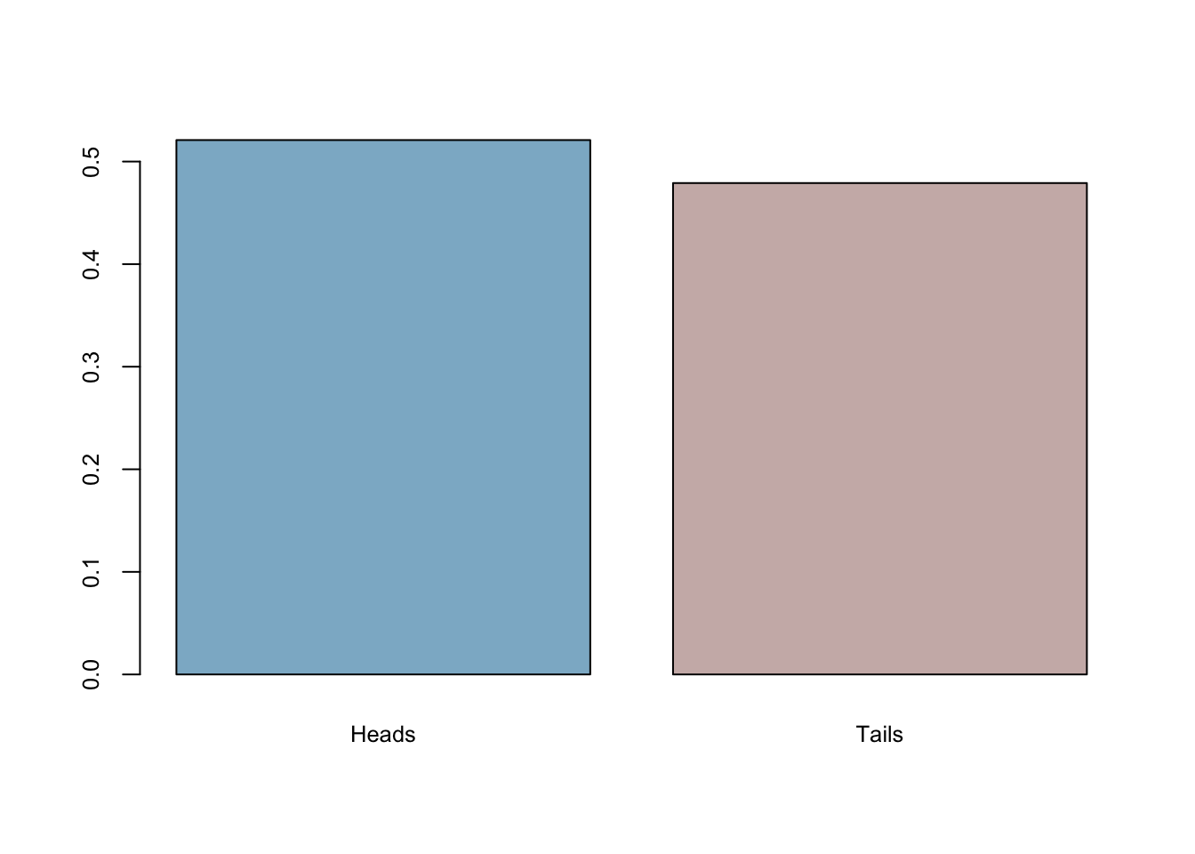
The true model generates heads 0.521 of the time. What if it always errs on the same side? In other words, what if it’s always bias towards heads in every sample with 501 flips? We will do our first simulation to answer it momentarily.
One more useful application:
sample(letters, 10, replace = TRUE)## [1] "p" "z" "o" "s" "c" "n" "a" "x" "a" "p"8.2 PDF’s in R
Here are the common probability distributions in R. Search help in R for more detail.
beta(shape1, shape2, ncp),
binom(size, prob),
chisq(df, ncp),
exp(rate),
gamma(shape, scale),
logis(location, scale),
norm(mean, sd),
pois(lambda),
t(df, ncp),
unif(min, max),
dnorm(x,) returns the density or the value on the y-axis of a probability distribution for a discrete value of x,
pnorm(q,) returns the cumulative density function (CDF) or the area under the curve to the left of an x value on a probability distribution curve,
qnorm(p,) returns the quantile value, i.e. the standardized z value for x,
rnorm(n,) returns a random simulation of size n
rnorm(6) # 6 values from a standard normal distribution## [1] -0.2645952 -0.9472983 0.7395213 0.8967787 -0.3460009 -1.7820571rnorm(10, mean = 50, sd = 19) # 10 values from a normal distribution## [1] 58.83389 12.93042 40.19385 59.29253 67.13847 62.16690 68.07297 38.61666
## [9] 24.71680 38.74801The binomial distribution is the distribution of the number of successes in n independent Bernoulli trials where a Bernoulli trial results in success or failure, with the probability of success = p
# A single Bernoulli trial (e.g. a coin flip) is given with size = 1.
rbinom(n = 1, size = 1, prob = 0.5)
## [1] 1# 10 trials for one flip (size = 1)
rbinom(n = 10, size = 1, prob = 0.5)## [1] 0 1 1 0 0 0 1 1 1 1# how many successes in 10 trials
rbinom(n = 1, size = 10, p = 0.5)## [1] 6So, a binomially distributed number is the same as the number of 1’s in n such Bernoulli numbers.
# 5 separate series of 10 trials
rbinom(n = 5, size = 10, p = 0.5)
## [1] 5 5 2 2 7These numbers shows how many 1’s we have out of 10 trials in each of 5 observations
Can we replicate our coin-flip example here with probability distributions? Yes, we can!
set.seed(123)
coins <- rbinom(n = 501, size = 1, p = 0.5)
mean(coins==0)
## [1] 0.5309381mean(coins)## [1] 0.4690619barplot(prop.table(table(coins)),
col = c("lightskyblue3","mistyrose3"),
cex.axis = 0.8, cex.names = 0.8)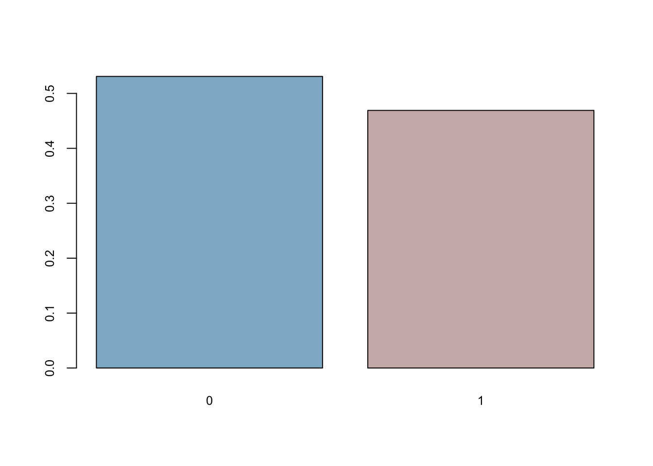
Uniform numbers are ones that are “equally likely” to be in the specified range. We use runif():
runif(n = 10, min = 0, max = 2) # Uniform distribution## [1] 0.7328829 0.5742003 0.1599458 0.7309085 0.3560276 1.0721074 1.0078974
## [8] 1.8900702 0.6826426 0.9294275Poisson distribution gives the likelihood of a certain number of events occurring in a given period of space or time. It can be used to estimate how likely it is that something will happen x number of times. For example, if the average number of people who buy cheeseburgers from a fast-food chain on a Friday night at a single restaurant location is 200, a Poisson distribution can answer questions such as, What is the probability that more than 300 people will buy burgers? The application of the Poisson distribution thereby enables managers to introduce optimal scheduling systems that would not work with, say, a normal distribution.
# Lambda = Average number of events
rpois(n = 10, lambda = 15) # Poisson distribution
## [1] 9 17 14 9 13 8 20 23 20 148.3 Simulation for statistical inference
Let’s apply a simulation to our coin flipping.
nsims <- 10000
nheads <- c()

for (i in 1:nsims){
  nheads[i] <- mean(rbinom(n = 501, size = 1, p = 0.5))
}

mean(nheads)
## [1] 0.4999669hist(nheads, col="blue", cex.axis = 0.75)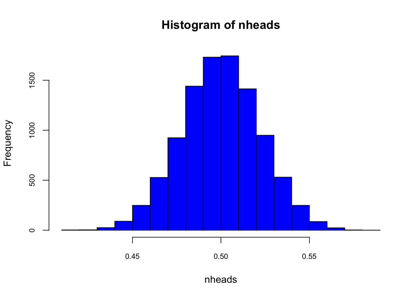
Here is another way for the same simulation:
nheads <- replicate(10000, mean(rbinom(n = 501, size = 1, p = 0.5)))
hist(nheads, col="pink",cex.axis = 0.75)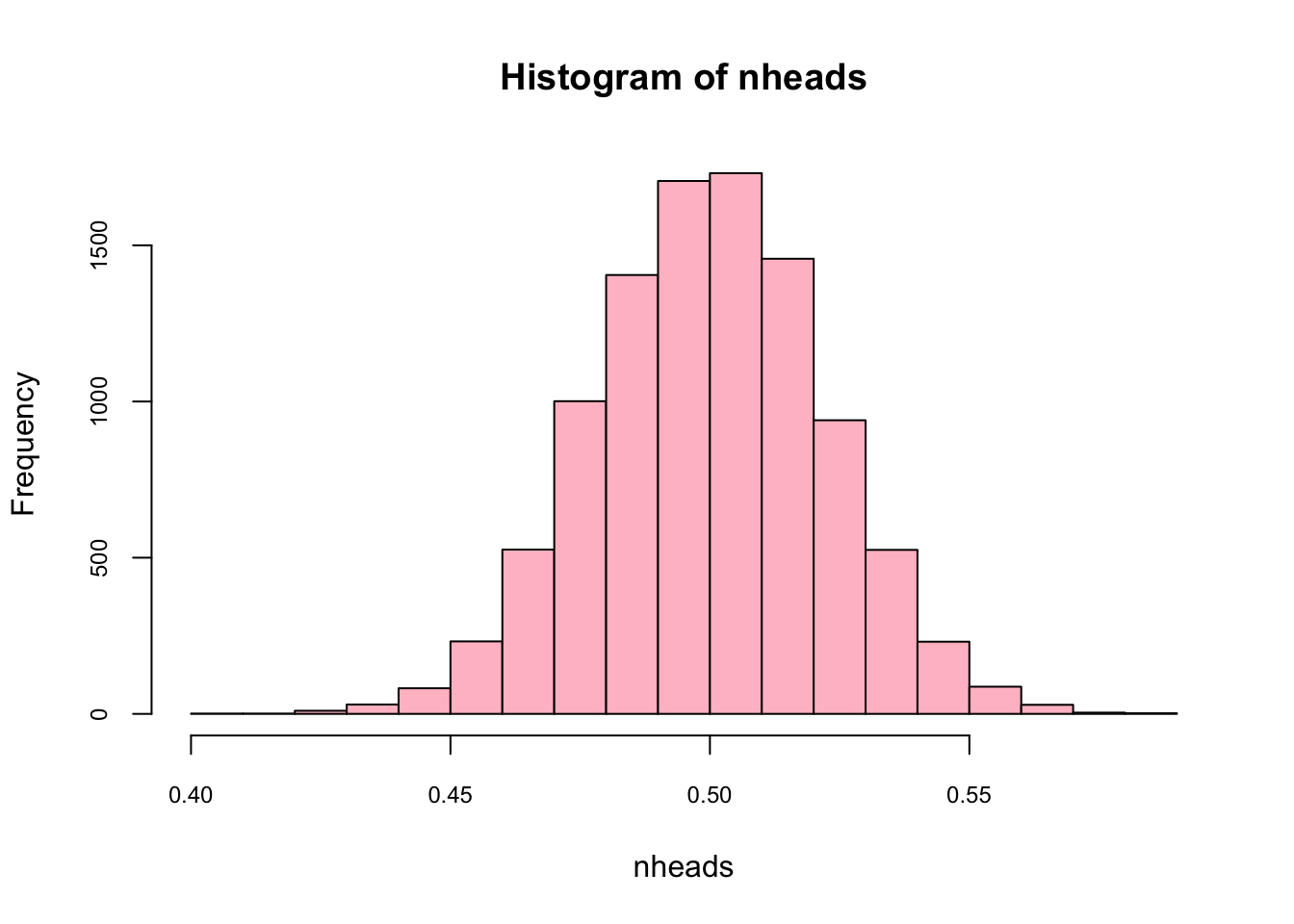
mean(nheads)## [1] 0.4999421What’s the 95% confidence interval for the mean? In other words, what’s the 95% CI for the mean of a randomly selected sample?
sd <- sd(nheads)
CI95 <- c(-1.96*sd+mean(nheads), 1.96*sd+mean(nheads))
CI95
## [1] 0.4563052 0.5435791What happens if we use a “wrong” estimator for the mean, like sum(heads)/300?
n.sims <- 10000
n.heads <- rep(NA, n.sims) # create vector to store simulations
for (i in 1:n.sims){
  n.heads[i] <- sum(rbinom(n = 501, size = 1, p = 0.5))/300
}
mean(n.heads)
## [1] 0.834594Because we are working with a simulation, it would be easy to show the result from this incorrect estimator.
8.4 Data Generating Model (DGM)
One of the major tasks of statistics is to obtain information about populations. In most of cases, the population is unknown and the only thing that is known for the researcher is a finite subset of observations drawn from the population. The main aim of the statistical analysis is to obtain information about the population through analysis of the sample. Since very little information is known about the population characteristics, one has to establish some assumptions about the behavior of this unknown population. For example, we can state the population regression function (PRF) as a data generating process (DGP). DGP can be expressed as the some of DGM plus the error term (\(u_i\)). For a pair of realizations \((x_i,y_i)\) from the random variables \((X,Y)\), we can write the following equalities:
\[ y_{i}=E\left(Y | X=x_{i}\right)+u_{i}=\text{DGM} + u_{i} = \alpha+\beta x_{i}+u_{i} =\text{DGP} \]
and
\[ E\left(u | X=x_{i}\right)=0 \]
This result implies that for \(X=x_i\), if the DGM is correctly specified, the divergences of all values of \(Y\) from the its conditional expectation \(E(Y\vert X=x_i)\) are averaged out. Hence, if DGM is not correctly specified, the error picks up those omitted variables and \(E\left(u | X=x_{i}\right)\neq0\).
In a regression analysis, the PRF includes DGM for \(y_i\), which is unknown to us. Because it is unknown, we must try to learn about it from a sample which is the only available data for us. If we assume that there is a specific PRF that generates the data, then given any estimator of \(\alpha\) and \(\beta\), namely \(\hat{\beta}\) and \(\hat{\alpha}\), we can estimate them from our sample with the sample regression function (SRF):
\[ \widehat{E\left(Y | X=x_{i}\right)}=\hat{y}_{i}=\hat{\alpha}+\hat{\beta} x_{i}, \quad i=1, \cdots, n \]
Hence,
\[ y_{i}=\hat{y}_{i}+\hat{u}_{i}, \quad i=1, \cdots, n \]
where \(\hat{u_i}\) is denoted the residuals from SRF.
With a data generating process (DGP) at hand, it is possible to create new simulated data, which could be viewed as an example of real-world data that a researcher would face. With the artificial data we generated, DGM is now known and the whole population is accessible. That is, we can test many models on different samples drawn from this population in order to see whether their inferential properties are in line with DGM. We’ll have several examples below.
Here is our DGM:
\[ Y_{i}=\beta_{1}+\beta_{2} X_{2 i}+\beta_{3} X_{3 i}+\beta_{4} X_{2 i} X_{3 i}+\beta_{5} X_{5 i}, \]
with the following coefficient vector: \(\beta = (12, -0.7, 34, -0.17, 5.4)\). Moreover \(x_2\) is a binary variable with values of 0 and 1 and \(x_5\) and \(x_3\) are highly correlated with \(\rho = 0.65\). When we add the error term, \(u\), which is independently and identically (i.i.d) distributed with \(N(0,1)\), we can get the whole population of 10,000 observations.
library(MASS)
N <- 10000
x_2 <- sample(c(0,1), N, replace = TRUE) #Dummy variable

#mvrnorm() creates a matrix of correlated variables
X_corr <- mvrnorm(N, mu = c(0,0), Sigma = matrix(c(1,0.65,0.65,1), ncol = 2),
               empirical = TRUE)

#We can check their correlation
cor(X_corr)
## [,1] [,2]
## [1,] 1.00 0.65
## [2,] 0.65 1.00#Each column is one of our variables
x_3 <- X_corr[,1]
x_5 <- X_corr[,2]
#interaction
x_23 <- x_2*x_3
# Now DGM
beta <- c(12, -0.7, 34, -0.17, 5.4)
dgm <- beta[1] + beta[2]*x_2 + beta[3]*x_3 + beta[4]*x_23 + beta[5]*x_5
#And our Y
y <- dgm + rnorm(N,0,1)
pop <- data.frame(y, x_2, x_3, x_23, x_5)
str(pop)## 'data.frame': 10000 obs. of 5 variables:
## $ y : num -49.2 16.8 -10.1 -50.2 93 ...
## $ x_2 : num 1 1 1 1 0 0 0 1 0 0 ...
## $ x_3 : num -1.575 0.307 -0.431 -1.487 2.159 ...
## $ x_23: num -1.575 0.307 -0.431 -1.487 0 ...
## $ x_5 : num -1.321 -0.692 -1.338 -1.726 1.3 ...#for better looking tables install.packages("stargazer")
library(stargazer)
stargazer(pop, type = "text", title = "Descriptive Statistics",
digits = 1, out = "table1.text")##
## Descriptive Statistics
## ============================================
## Statistic N Mean St. Dev. Min Max
## --------------------------------------------
## y 10,000 11.7 37.7 -143.1 164.3
## x_2 10,000 0.5 0.5 0 1
## x_3 10,000 0.0 1.0 -3.9 3.9
## x_23 10,000 0.002 0.7 -3.2 3.7
## x_5 10,000 -0.0 1.0 -3.8 3.6
## --------------------------------------------#The table will be saved in the working directory too
#with whatever name you write in the out option.
#You can open this file with any word processorNow we are going to sample this population and run a SRF.
library(stargazer)

n <- 500 #sample size
ind <- sample(nrow(pop), n, replace = FALSE)
sample <- pop[ind, ]
str(sample)
## 'data.frame': 500 obs. of 5 variables:
## $ y : num 40.8 55.8 -11.1 17.9 20.5 ...
## $ x_2 : num 1 0 0 0 0 0 1 0 1 0 ...
## $ x_3 : num 0.9187 1.177 -0.5007 0.3275 0.0758 ...
## $ x_23: num 0.919 0 0 0 0 ...
## $ x_5 : num -0.221 0.692 -0.724 -0.606 1.417 ...model <- lm(y ~ ., data = sample)
stargazer(model, type = "text", title = "G O O D - M O D E L",
dep.var.labels = "Y",
digits = 3)##
## G O O D - M O D E L
## ================================================
## Dependent variable:
## ----------------------------
## Y
## ------------------------------------------------
## x_2 -0.714***
## (0.089)
##
## x_3 34.029***
## (0.070)
##
## x_23 -0.164*
## (0.089)
##
## x_5 5.344***
## (0.055)
##
## Constant 11.945***
## (0.061)
##
## ------------------------------------------------
## Observations 500
## R2 0.999
## Adjusted R2 0.999
## Residual Std. Error 0.992 (df = 495)
## F Statistic 177,153.800*** (df = 4; 495)
## ================================================
## Note: *p<0.1; **p<0.05; ***p<0.01As you can see the coefficients are very close to our “true” coefficients specified in DGM. Now we can test what happens if we omit \(x_5\) in our SRF and estimate it.
library(stargazer)

n <- 500 #sample size
sample <- pop[sample(nrow(pop), n, replace = FALSE), ]
str(sample)
## 'data.frame': 500 obs. of 5 variables:
## $ y : num 22.46 6.48 35.52 32.34 -16.7 ...
## $ x_2 : num 1 1 0 1 1 1 0 1 1 0 ...
## $ x_3 : num 0.2913 0.0582 0.3794 0.7569 -0.6862 ...
## $ x_23: num 0.2913 0.0582 0 0.7569 -0.6862 ...
## $ x_5 : num 0.146 -1.156 1.972 -0.523 -0.518 ...model_bad <- lm(y ~ x_2 + x_3 + x_23, data = sample)
stargazer(model_bad, type = "text", title = "B A D - M O D E L",
dep.var.labels = "Y",
digits = 3)##
## B A D - M O D E L
## ===============================================
## Dependent variable:
## ---------------------------
## Y
## -----------------------------------------------
## x_2 -0.485
## (0.377)
##
## x_3 37.569***
## (0.266)
##
## x_23 -0.501
## (0.387)
##
## Constant 11.886***
## (0.271)
##
## -----------------------------------------------
## Observations 500
## R2 0.987
## Adjusted R2 0.987
## Residual Std. Error 4.205 (df = 496)
## F Statistic 12,481.320*** (df = 3; 496)
## ===============================================
## Note: *p<0.1; **p<0.05; ***p<0.01Now it seems that none of the coefficients are as good as before, except for the intercept. This is a so-called omitted variable bias (OVB) problem, also known as a model underfitting or specification error. Would it be a problem for only one sample? We can simulate the results many times and see whether on average \(\hat{\beta_3}\) is biased or not.
n.sims <- 500
n <- 500 #sample size
beta_3 <- c(0)

for (i in 1:n.sims){
  set.seed(i)
  sample <- pop[sample(nrow(pop), n, replace = FALSE), ]
  model_bad <- lm(y ~ x_2 + x_3 + x_23, data = sample)
  beta_3[i] <- model_bad$coefficients["x_3"]
}
summary(beta_3)
## Min. 1st Qu. Median Mean 3rd Qu. Max.
## 36.76 37.32 37.50 37.50 37.67 38.26As we can see the OVB problem is not a problem in one sample. We withdrew a sample and estimated the same underfitting model 500 times with a simulation. Hence, we collected 500 \(\hat{\beta_3}\). The average is 37.58. If we do the same simulation with a model that is correctly specified, you can see the results: the average of 500 \(\hat{\beta_3}\) is 34, which is the “correct”true” coefficient in our DGM.
n.sims <- 500
n <- 500 #sample size
beta_3 <- c(NA, n.sims)

for (i in 1:n.sims){
  sample <- pop[sample(nrow(pop), n, replace = FALSE), ]
  model_good <- lm(y ~ x_2 + x_3 + x_23 + x_5, data = sample)
  beta_3[i] <- model_good$coefficients["x_3"]
}
summary(beta_3)
## Min. 1st Qu. Median Mean 3rd Qu. Max.
## 33.79 33.94 33.99 33.99 34.04 34.198.5 Bootstrapping
Bootstrapping is the process of resampling with replacement with an equal probabilities. With bootstrapping, we can calculate a statistic (e.g. the mean) from each bootstrapped sample repeated thousands of times and estimate a precise/accurate uncertainty of the mean (confidence interval) of the data’s distribution.
Generally bootstrapping follows the same basic steps:
- Resample a given data set a specified number of times,
- Calculate a specific statistic from each sample,
- Find the standard deviation of the distribution of that statistic.
In the following bootstrapping example we would like to obtain a standard error for the estimate of the mean. We will be using the lapply(), sapply() functions in combination with the sample function. (see this link for more details: https://stats.idre.ucla.edu/r/library/r-library-introduction-to-bootstrapping/)(UCLA_2021?)
Let’s create a data set by taking 100 observations from a normal distribution with mean 5 and standard deviation 3:
set.seed(123)
data <- rnorm(100, 5, 3)

#obtaining 20 bootstrap samples and storing in a list
resamples <- lapply(1:20, function(i) sample(data, replace = T))

resamples[1]
## [[1]]
## [1] 8.76144476 3.11628177 4.02220524 10.36073941 6.30554447 9.10580685
## [7] 2.93597415 3.60003394 3.58162578 6.34462934 5.71619521 7.06592076
## [13] 4.91435973 4.34607526 7.33989536 4.37624817 5.37156273 6.93312965
## [19] 8.67224539 4.32268704 1.20481630 1.63067425 4.33854031 5.91058592
## [25] 4.14568098 1.63067425 11.15025406 -1.92750663 11.50686790 4.11478555
## [31] 7.06592076 8.62388599 5.33204815 10.36073941 8.29051704 7.68537698
## [37] 3.85858700 3.85858700 3.66301409 4.02220524 -1.92750663 6.15584120
## [43] 2.93944144 6.38274862 6.38274862 6.75384125 6.13891845 2.87239771
## [49] 2.81332631 4.00037785 9.10580685 1.92198666 -0.06007993 7.68537698
## [55] 0.35374159 1.58558919 3.66301409 4.87138863 9.10580685 4.14568098
## [61] 8.67224539 3.12488220 4.91435973 -0.06007993 6.38274862 3.12488220
## [67] 8.29051704 8.44642286 4.11478555 6.93312965 2.81332631 0.35374159
## [73] 8.01721557 1.92198666 5.33204815 10.14519496 7.98051157 3.31857306
## [79] 8.44642286 6.75384125 5.01729256 1.58558919 -0.06007993 7.51336113
## [85] 4.33854031 6.38274862 5.64782471 -0.06007993 2.91587906 6.93312965
## [91] 10.14519496 3.11628177 6.27939266 5.71619521 6.49355143 1.94427385
## [97] 6.66175296 0.35374159 3.58162578 7.46474324Here is another way to do the same thing:
set.seed(123)
data <- rnorm(100, 5, 3)
resamples_2 <- matrix(NA, nrow = 100, ncol = 20)

for (i in 1:20) {
  resamples_2[,i] <- sample(data, 100, replace = TRUE)
}

dim(resamples_2)
## [1] 100 20#display the first of the bootstrap samples
resamples_2[, 1]## [1] 8.76144476 3.11628177 4.02220524 10.36073941 6.30554447 9.10580685
## [7] 2.93597415 3.60003394 3.58162578 6.34462934 5.71619521 7.06592076
## [13] 4.91435973 4.34607526 7.33989536 4.37624817 5.37156273 6.93312965
## [19] 8.67224539 4.32268704 1.20481630 1.63067425 4.33854031 5.91058592
## [25] 4.14568098 1.63067425 11.15025406 -1.92750663 11.50686790 4.11478555
## [31] 7.06592076 8.62388599 5.33204815 10.36073941 8.29051704 7.68537698
## [37] 3.85858700 3.85858700 3.66301409 4.02220524 -1.92750663 6.15584120
## [43] 2.93944144 6.38274862 6.38274862 6.75384125 6.13891845 2.87239771
## [49] 2.81332631 4.00037785 9.10580685 1.92198666 -0.06007993 7.68537698
## [55] 0.35374159 1.58558919 3.66301409 4.87138863 9.10580685 4.14568098
## [61] 8.67224539 3.12488220 4.91435973 -0.06007993 6.38274862 3.12488220
## [67] 8.29051704 8.44642286 4.11478555 6.93312965 2.81332631 0.35374159
## [73] 8.01721557 1.92198666 5.33204815 10.14519496 7.98051157 3.31857306
## [79] 8.44642286 6.75384125 5.01729256 1.58558919 -0.06007993 7.51336113
## [85] 4.33854031 6.38274862 5.64782471 -0.06007993 2.91587906 6.93312965
## [91] 10.14519496 3.11628177 6.27939266 5.71619521 6.49355143 1.94427385
## [97] 6.66175296 0.35374159 3.58162578 7.46474324Calculating the mean for each bootstrap sample:
colMeans(resamples_2)## [1] 5.095470 5.611315 5.283893 4.930731 4.804722 5.187125 4.946582 4.952693
## [9] 5.470162 5.058354 4.790996 5.357154 5.479364 5.366046 5.454458 5.474732
## [17] 5.566421 5.229395 5.111966 5.262666#and the mean of all means
mean(colMeans(resamples_2))## [1] 5.221712Calculating the standard deviation of the distribution of means:
sqrt(var(colMeans(resamples_2)))## [1] 0.25232548.6 Monty Hall - Fun example
The Monty Hall problem is a well-known brain teaser based on the American television game show Let’s Make a Deal and named after its original host, Monty Hall. Here is an excerpt from Wikipedia
Hall’s name is used in a probability puzzle known as the “Monty Hall problem”. The name was conceived by statistician Steve Selvin who used the title in describing a probability problem to Scientific American in 1975 based on one of the games on Let’s Make a Deal, and more popularized when it was presented in a weekly national newspaper column by Marilyn vos Savant in 1990.
A host (“Monty”) provides a player with three doors, one containing a valuable prize and the other two containing a “gag”, valueless prize. The contestant is offered a choice of one of the doors without knowledge of the content behind them. “Monty”, who knows which door has the prize, opens a door that the player did not select that has a gag prize, and then offers the player the option to switch from their choice to the other remaining unopened door. The probability problem arises from asking if the player should switch to the unrevealed door.
Mathematically, the problem shows that a player switching to the other door has a 2/3 chance of winning under standard conditions, but this is a counterintuitive effect of switching one’s choice of doors, and the problem gained wide attention due to conflicting views following vos Savant’s publication, with many asserting that the probability of winning had dropped to 1/2 if one switched. A number of other solutions become possible if the problem setup is outside of the “standard conditions” defined by vos Savant: that the host equally selects one of the two gag prize doors if the player had first picked the winning prize, and the offer to switch is always presented.
Hall gave an explanation of the solution to that problem in an interview with The New York Times reporter John Tierney in 1991. In the article, Hall pointed out that because he had control over the way the game progressed, playing on the psychology of the contestant, the theoretical solution did not apply to the show’s actual gameplay. He said he was not surprised at the experts’ insistence that the probability was 1 out of 2. “That’s the same assumption contestants would make on the show after I showed them there was nothing behind one door,” he said. “They’d think the odds on their door had now gone up to 1 in 2, so they hated to give up the door no matter how much money I offered. By opening that door we were applying pressure. We called it the Henry James treatment. It was ‘The Turn of the Screw.’” Hall clarified that as a game show host he was not required to follow the rules of the puzzle as Marilyn vos Savant often explains in her weekly column in Parade, and did not always allow a person the opportunity to switch. For example, he might open their door immediately if it was a losing door, might offer them money to not switch from a losing door to a winning door, or might only allow them the opportunity to switch if they had a winning door. “If the host is required to open a door all the time and offer you a switch, then you should take the switch,” he said. “But if he has the choice whether to allow a switch or not, beware. Caveat emptor. It all depends on his mood.”
Many readers of vos Savant’s column refused to believe switching is beneficial despite her explanation. After the problem appeared in Parade, approximately 10,000 readers, including nearly 1,000 with PhDs, wrote to the magazine, most of them claiming vos Savant was wrong. Even when given explanations, simulations, and formal mathematical proofs, many people still do not accept that switching is the best strategy. Paul Erdős, one of the most prolific mathematicians in history, remained unconvinced until he was shown a computer simulation demonstrating the predicted result.
The given probabilities depend on specific assumptions about how the host and contestant choose their doors. A key insight is that, under these standard conditions, there is more information about doors 2 and 3 that was not available at the beginning of the game, when door 1 was chosen by the player: the host’s deliberate action adds value to the door he did not choose to eliminate, but not to the one chosen by the contestant originally. Another insight is that switching doors is a different action than choosing between the two remaining doors at random, as the first action uses the previous information and the latter does not. Other possible behaviors than the one described can reveal different additional information, or none at all, and yield different probabilities.
Here is the simple Bayes rule: \(Pr(A|B) = Pr(B|A)Pr(A)/Pr(B)\).
Let’s play it: The player picks Door 1, Monty Hall opens Door 3. My question is this:
\(Pr(CAR = 1|Open = 3) < Pr(CAR = 2|Open = 3)\)?
If this is true the player should always switch. Here is the Bayesian answer:
\(Pr(Car=1|Open=3) = Pr(Open=3|Car=1)Pr(Car=1)/Pr(Open=3)\) = 1/2 x (1/3) / (1/2) = 1/3
Let’s see each number. Given that the player picks Door 1, if the car is behind Door 1, Monty should be indifferent between opening Doors 2 and 3. So the first term is 1/2. The second term is easy: Probability that the car is behind Door 1 is 1/3. The third term is also simple and usually overlooked. This is not a conditional probability. If the car were behind Door 2, the probability that Monty opens Door 3 would be 1. And this explains why the second option is different, below:
\(Pr(Car=2|Open=3) = Pr(Open=3|Car=2)Pr(Car=2)/Pr(Open=3)\) = 1 x (1/3) / (1/2) = 2/3

Image taken from http://media.graytvinc.com/images/690*388/mon+tyhall.jpg
Step 2: Define all possible door combinations
3 doors, the first one has the car. All possible outcomes for the game:
outcomes <- c(123,132,213,231,312,321)Step 3: Create empty containers where you store the outcomes from each game
car <- rep(0, n)
goat1 <- rep(0, n)
goat2 <- rep(0, n)
choice <- rep(0,n)
monty <- rep(0, n)
winner <- rep(0, n)
Step 4: Loop
for (i in 1:n){
  doors <- sample(outcomes,1) #The game's door combination
  car[i] <- substring(doors, first = c(1,2,3), last = c(1,2,3))[1] #the right door
  goat1[i] <- substring(doors, first = c(1,2,3), last = c(1,2,3))[2] #The first wrong door
  goat2[i] <- substring(doors, first = c(1,2,3), last = c(1,2,3))[3] #The second wrong door

  #Person selects a random door
  choice[i] <- sample(1:3,1)

  #Now Monty opens a door
  if (choice[i] == car[i])
    {monty[i] = sample(c(goat1[i],goat2[i]),1)}
  else if (choice[i] == goat1[i])
    {monty[i] = goat2[i]}
  else
    {monty[i] = goat1[i]}

  # 1 represents the stayer who remains by her initial choice
  # 2 represents the switcher who changes her initial choice
  if (choice[i] == car[i]){winner[i] = 1} else {winner[i] = 2}
}
Step 5: Chart
hist(winner, breaks = 2, main = "Who would win the most?",
     ylim = c(0,70000), labels = c("Stayer", "Switcher"),
     col = c("aliceblue", "pink"),
     cex.axis = 0.75, cex.lab = 0.75, cex.main = 0.85)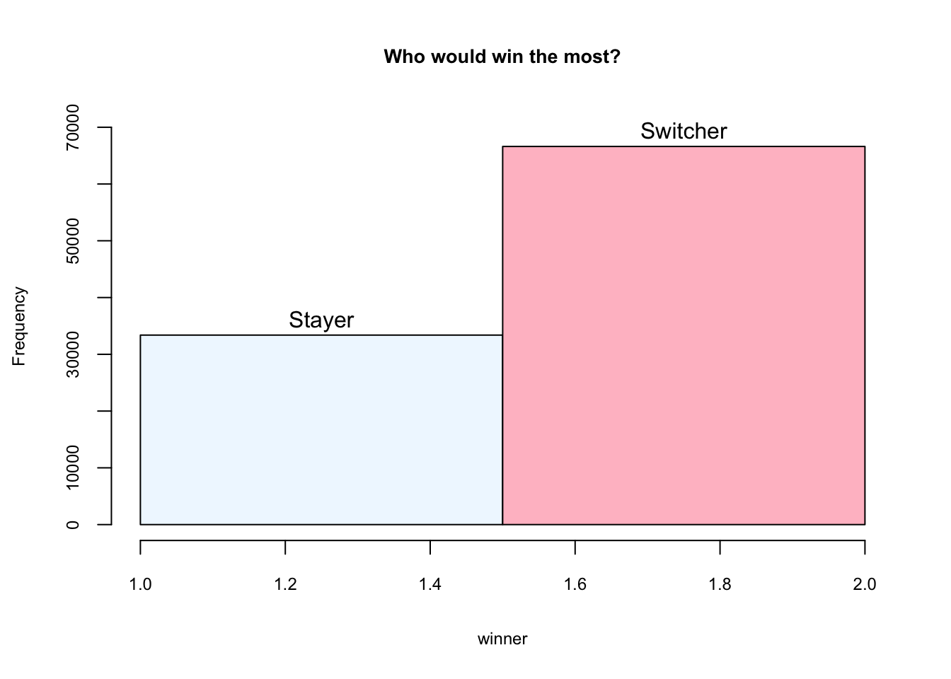
The simulation is inspired by https://theressomethingaboutr.wordpress.com/2019/02/12/in-memory-of-monty-hall/ (Rajter_2019?)