Chapter 31 Factor Analysis
Factor analysis and Principal Component Analysis (PCA) both involve reducing the dimensionality of a dataset, but they are not the same. PCA is a mathematical technique that transforms a dataset of possibly correlated variables into a smaller set of uncorrelated variables known as principal components. The principal components are linear combinations of the original variables, and each principal component accounts for as much of the variation in the data as possible.
Factor Analysis (FA) is a method for modeling observed variables, and their covariance structure, in terms of a smaller number of underlying latent (unobserved) “factors”. In FA the observed variables are modeled as linear functions of the “factors.” In PCA, we create new variables that are linear combinations of the observed variables. In both PCA and FA, the dimension of the data is reduced.
The main difference between FA and PCA lies in their objectives. PCA aims to reduce the number of variables by identifying the most important components, while factor analysis aims to identify the underlying factors that explain the correlations among the variables. Therefore, PCA is more commonly used for data reduction or data compression, while factor analysis is more commonly used for exploring the relationships among variables.
As shown below, a factor model can be represented by as a series of multiple regressions, where each \(X_{i}\) (\(i = 1, \cdots, p\)) is a function of \(m\) number of unobservable common factors \(f_{i}\):
\[ \begin{gathered} X_{1}=\mu_{1}+\beta_{11} f_{1}+\beta_{12} f_{2}+\cdots+\beta_{1m} f_{m}+\epsilon_{1} \\ X_{2}=\mu_{2}+\beta_{21} f_{1}+\beta_{22} f_{2}+\cdots+\beta_{2 m} f_{m}+\epsilon_{2} \\ \vdots \\ X_{p}=\mu_{p}+\beta_{p 1} f_{1}+\beta_{p 2} f_{2}+\cdots+\beta_{p m} f_{m}+\epsilon_{p} \end{gathered} \]
where \(\mathrm{E}\left(X_i\right)=\mu_i\), \(\epsilon_{i}\) are called the specific factors. The coefficients, \(\beta_{i j},\) are the factor loadings. We can expressed all of them in a matrix notation.
\[\begin{equation} \mathbf{X}=\boldsymbol{\mu}+\mathbf{L f}+\boldsymbol{\epsilon} \end{equation}\]
where
\[ \mathbf{L}=\left(\begin{array}{cccc} \beta_{11} & \beta_{12} & \ldots & \beta_{1 m} \\ \beta_{21} & \beta_{22} & \ldots & \beta_{2 m} \\ \vdots & \vdots & & \vdots \\ \beta_{p 1} & \beta_{p 2} & \ldots & \beta_{p m} \end{array}\right) \]
There are multiple assumptions:
- \(E\left(\epsilon_{i}\right)=0\) and \(\operatorname{var}\left(\epsilon_{i}\right)=\psi_{i}\), which is called as “specific variance”,
- \(E\left(f_{i}\right)=0\) and \(\operatorname{var}\left(f_{i}\right)=1\),
- \(\operatorname{cov}\left(f_{i}, f_{j}\right)=0\) for \(i \neq j\),
- \(\operatorname{cov}\left(\epsilon_{i}, \epsilon_{j}\right)=0\) for \(i \neq j\),
- \(\operatorname{cov}\left(\epsilon_{i}, f_{j}\right)=0\),
Given these assumptions, the variance of \(X_i\) can be expressed as
\[ \operatorname{var}\left(X_{i}\right)=\sigma_{i}^{2}=\sum_{j=1}^{m} \beta_{i j}^{2}+\psi_{i} \]
There are two sources of the variance in \(X_i\): \(\sum_{j=1}^{m} \beta_{i j}^{2}\), which is called the Communality for variable \(i\), and specific variance, \(\psi_{i}\).
Moreover,
- \(\operatorname{cov}\left(X_{i}, X_{j}\right)=\sigma_{i j}=\sum_{k=1}^{m} l_{i k} l_{j k}\),
- \(\operatorname{cov}\left(X_{i}, f_{j}\right)=l_{i j}\)
The factor model for our variance-covariance matrix of \(\mathbf{X}\) can then be expressed as:
\[ \begin{equation} \operatorname{var-cov}(\mathbf{X}) = \Sigma=\mathbf{L L}^{\prime}+\mathbf{\Psi} \end{equation} \]
which is the sum of the shared variance with another variable, \(\mathbf{L} \mathbf{L}^{\prime}\) (the common variance or communality) and the unique variance, \(\mathbf{\Psi}\), inherent to each variable (specific variance)
We need to look at \(\mathbf{L L}^{\prime}\), where \(\mathbf{L}\) is the \(p \times m\) matrix of loadings. In general, we want to have \(m \ll p\).
The \(i^{\text {th }}\) diagonal element of \(\mathbf{L L}^{\prime}\), the sum of the squared loadings, is called the \(i^{\text {th }}\) communality. The communality values represent the percent of variability explained by the common factors. The sizes of the communalities and/or the specific variances can be used to evaluate the goodness of fit.
To estimate factor loadings with PCA, we first calculate the principal components of the data, and then compute the factor loadings using the eigenvectors of the correlation matrix of the standardized data. When PCA is used, the matrix of estimated factor loadings, \(\mathbf{L},\) is given by:
\[ \widehat{\mathbf{L}}=\left[\begin{array}{lll} \sqrt{\hat{\lambda}_1} \hat{\mathbf{v}}_1 & \sqrt{\hat{\lambda}_2} \hat{\mathbf{v}}_2 & \ldots \sqrt{\hat{\lambda}_m} \hat{\mathbf{v}}_m \end{array}\right] \]
where
\[ \hat{\beta}_{i j}=\hat{\mathbf{v}}_{i j} \sqrt{\hat{\lambda}_j} \] where \(i\) is the index of the original variable, \(j\) is the index of the principal component, eigenvector \((i,j)\) is the \(i\)-th component of the \(j\)-th eigenvector of the correlation matrix, eigenvalue \((j)\) is the \(j\)-th eigenvalue of the correlation matrix
This method tries to find values of the loadings that bring the estimate of the total communality close to the total of the observed variances. The covariances are ignored. Remember, the communality is the part of the variance of the variable that is explained by the factors. So a larger communality means a more successful factor model in explaining the variable.
Let’s have an example. The data set is called bfi and comes from the psych package.
The data includes 25 self-reported personality items from the International Personality Item Pool, gender, education level, and age for 2800 subjects. The personality items are split into 5 categories: Agreeableness (A), Conscientiousness (C), Extraversion (E), Neuroticism (N), Openness (O). Each item was answered on a six point scale: 1 Very Inaccurate to 6 Very Accurate.
library(psych)
library(GPArotation)
data("bfi")
str(bfi)
## 'data.frame': 2800 obs. of 28 variables:
## $ A1 : int 2 2 5 4 2 6 2 4 4 2 ...
## $ A2 : int 4 4 4 4 3 6 5 3 3 5 ...
## $ A3 : int 3 5 5 6 3 5 5 1 6 6 ...
## $ A4 : int 4 2 4 5 4 6 3 5 3 6 ...
## $ A5 : int 4 5 4 5 5 5 5 1 3 5 ...
## $ C1 : int 2 5 4 4 4 6 5 3 6 6 ...
## $ C2 : int 3 4 5 4 4 6 4 2 6 5 ...
## $ C3 : int 3 4 4 3 5 6 4 4 3 6 ...
## $ C4 : int 4 3 2 5 3 1 2 2 4 2 ...
## $ C5 : int 4 4 5 5 2 3 3 4 5 1 ...
## $ E1 : int 3 1 2 5 2 2 4 3 5 2 ...
## $ E2 : int 3 1 4 3 2 1 3 6 3 2 ...
## $ E3 : int 3 6 4 4 5 6 4 4 NA 4 ...
## $ E4 : int 4 4 4 4 4 5 5 2 4 5 ...
## $ E5 : int 4 3 5 4 5 6 5 1 3 5 ...
## $ N1 : int 3 3 4 2 2 3 1 6 5 5 ...
## $ N2 : int 4 3 5 5 3 5 2 3 5 5 ...
## $ N3 : int 2 3 4 2 4 2 2 2 2 5 ...
## $ N4 : int 2 5 2 4 4 2 1 6 3 2 ...
## $ N5 : int 3 5 3 1 3 3 1 4 3 4 ...
## $ O1 : int 3 4 4 3 3 4 5 3 6 5 ...
## $ O2 : int 6 2 2 3 3 3 2 2 6 1 ...
## $ O3 : int 3 4 5 4 4 5 5 4 6 5 ...
## $ O4 : int 4 3 5 3 3 6 6 5 6 5 ...
## $ O5 : int 3 3 2 5 3 1 1 3 1 2 ...
## $ gender : int 1 2 2 2 1 2 1 1 1 2 ...
## $ education: int NA NA NA NA NA 3 NA 2 1 NA ...
## $ age : int 16 18 17 17 17 21 18 19 19 17 ...To get rid of missing observations and the last three variables,
df <- bfi[complete.cases(bfi[, 1:25]), 1:25]The first decision that we need make is the number of factors that we will need to extract. For \(p=25\), the variance-covariance matrix \(\Sigma\) contains \[ \frac{p(p+1)}{2}=\frac{25 \times 26}{2}=325 \] unique elements or entries. With \(m\) factors, the number of parameters in the factor model would be
\[ p(m+1)=25(m+1) \]
Taking \(m=5\), we have 150 parameters in the factor model. How do we choose \(m\)? Although it is common to look at the results of the principal components analysis, often in social sciences, the underlying theory within the field of study indicates how many factors to expect.
scree(df)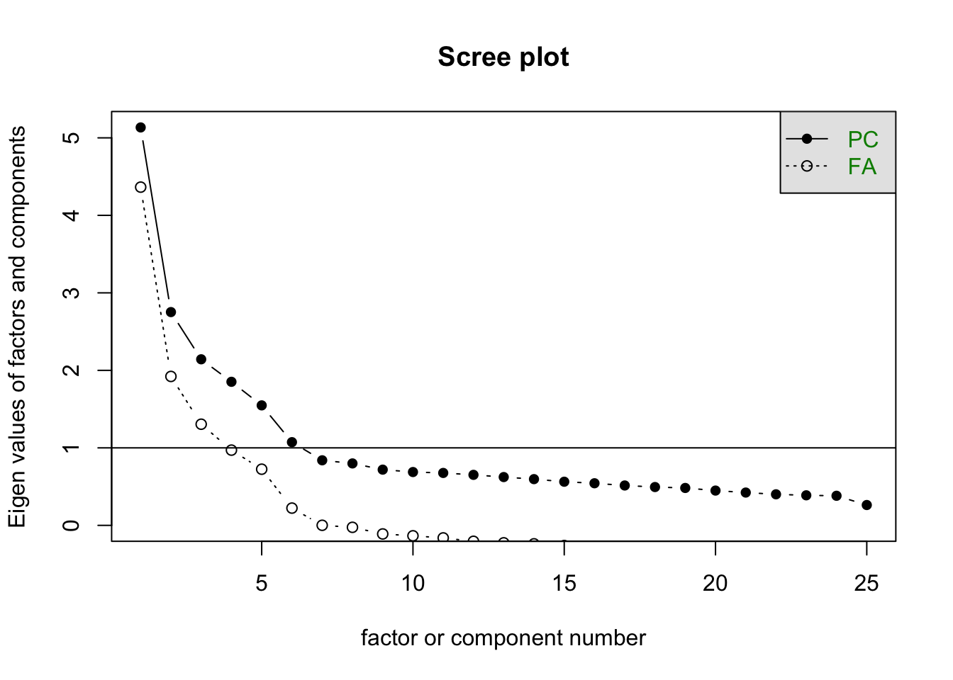
Let’s use the factanal() function of the build-in stats package, which performs maximum likelihood estimation.
pa.out <- factanal(df, factors = 5)
pa.out
##
## Call:
## factanal(x = df, factors = 5)
##
## Uniquenesses:
## A1 A2 A3 A4 A5 C1 C2 C3 C4 C5 E1 E2 E3
## 0.830 0.576 0.466 0.691 0.512 0.660 0.569 0.677 0.510 0.557 0.634 0.454 0.558
## E4 E5 N1 N2 N3 N4 N5 O1 O2 O3 O4 O5
## 0.468 0.592 0.271 0.337 0.478 0.507 0.664 0.675 0.744 0.518 0.752 0.726
##
## Loadings:
## Factor1 Factor2 Factor3 Factor4 Factor5
## A1 0.104 -0.393
## A2 0.191 0.144 0.601
## A3 0.280 0.110 0.662
## A4 0.181 0.234 0.454 -0.109
## A5 -0.124 0.351 0.580
## C1 0.533 0.221
## C2 0.624 0.127 0.140
## C3 0.554 0.122
## C4 0.218 -0.653
## C5 0.272 -0.190 -0.573
## E1 -0.587 -0.120
## E2 0.233 -0.674 -0.106 -0.151
## E3 0.490 0.315 0.313
## E4 -0.121 0.613 0.363
## E5 0.491 0.310 0.120 0.234
## N1 0.816 -0.214
## N2 0.787 -0.202
## N3 0.714
## N4 0.562 -0.367 -0.192
## N5 0.518 -0.187 0.106 -0.137
## O1 0.182 0.103 0.524
## O2 0.163 -0.113 0.102 -0.454
## O3 0.276 0.153 0.614
## O4 0.207 -0.220 0.144 0.368
## O5 -0.512
##
## Factor1 Factor2 Factor3 Factor4 Factor5
## SS loadings 2.687 2.320 2.034 1.978 1.557
## Proportion Var 0.107 0.093 0.081 0.079 0.062
## Cumulative Var 0.107 0.200 0.282 0.361 0.423
##
## Test of the hypothesis that 5 factors are sufficient.
## The chi square statistic is 1490.59 on 185 degrees of freedom.
## The p-value is 1.22e-202The first chunk provides the “uniqueness” (specific variance) for each variable, which range from 0 to 1 . The uniqueness explains the proportion of variability, which cannot be explained by a linear combination of the factors. That’s why it’s referred to as noise. This is the \(\hat{\Psi}\) in the equation above. A high uniqueness for a variable implies that the factors are not the main source of its variance.
The next section reports the loadings ranging from \(-1\) to \(1.\) This is the \(\hat{\mathbf{L}}\) in the equation (31.2) above. Variables with a high loading are well explained by the factor. Note that R does not print loadings less than \(0.1\).
The communalities for the \(i^{t h}\) variable are computed by taking the sum of the squared loadings for that variable. This is expressed below:
\[ \hat{h}_i^2=\sum_{j=1}^m \hat{l}_{i j}^2 \]
A well-fit factor model has low values for uniqueness and high values for communality. One way to calculate the communality is to subtract the uniquenesses from 1.
apply(pa.out$loadings ^ 2, 1, sum) # communality## A1 A2 A3 A4 A5 C1 C2 C3
## 0.1703640 0.4237506 0.5337657 0.3088959 0.4881042 0.3401202 0.4313729 0.3227542
## C4 C5 E1 E2 E3 E4 E5 N1
## 0.4900773 0.4427531 0.3659303 0.5459794 0.4422484 0.5319941 0.4079732 0.7294156
## N2 N3 N4 N5 O1 O2 O3 O4
## 0.6630751 0.5222584 0.4932099 0.3356293 0.3253527 0.2558864 0.4815981 0.2484000
## O5
## 0.27405961 - apply(pa.out$loadings ^ 2, 1, sum) # uniqueness## A1 A2 A3 A4 A5 C1 C2 C3
## 0.8296360 0.5762494 0.4662343 0.6911041 0.5118958 0.6598798 0.5686271 0.6772458
## C4 C5 E1 E2 E3 E4 E5 N1
## 0.5099227 0.5572469 0.6340697 0.4540206 0.5577516 0.4680059 0.5920268 0.2705844
## N2 N3 N4 N5 O1 O2 O3 O4
## 0.3369249 0.4777416 0.5067901 0.6643707 0.6746473 0.7441136 0.5184019 0.7516000
## O5
## 0.7259404The table under the loadings reports the proportion of variance explained by each factor. Proportion Var shows the proportion of variance explained by each factor. The row Cumulative Var is the cumulative Proportion Var. Finally, the row SS loadings reports the sum of squared loadings. This can be used to determine a factor worth keeping (Kaiser Rule).
The last section of the output reports a significance test: The null hypothesis is that the number of factors in the model is sufficient to capture the full dimensionality of the data set. Hence, in our example, we fitted not an appropriate model.
Finally, we may compare estimated correlation matrix, \(\hat{\Sigma}\) and the observed correlation matrix:
Lambda <- pa.out$loadings
Psi <- diag(pa.out$uniquenesses)
Sigma_hat <- Lambda %*% t(Lambda) + Psi
head(Sigma_hat)
## A1 A2 A3 A4 A5 C1
## A1 1.00000283 -0.2265272 -0.2483489 -0.1688548 -0.2292686 -0.03259104
## A2 -0.22652719 0.9999997 0.4722224 0.3326049 0.4275597 0.13835721
## A3 -0.24834886 0.4722224 1.0000003 0.3686079 0.4936403 0.12936294
## A4 -0.16885485 0.3326049 0.3686079 1.0000017 0.3433611 0.13864850
## A5 -0.22926858 0.4275597 0.4936403 0.3433611 1.0000000 0.11450065
## C1 -0.03259104 0.1383572 0.1293629 0.1386485 0.1145007 1.00000234
## C2 C3 C4 C5 E1 E2
## A1 -0.04652882 -0.04791267 0.02951427 0.03523371 0.02815444 0.0558511
## A2 0.17883430 0.15482391 -0.12081021 -0.13814633 -0.18266118 -0.2297604
## A3 0.16516097 0.14465370 -0.11034318 -0.14189597 -0.24413210 -0.2988190
## A4 0.18498354 0.18859903 -0.18038121 -0.21194824 -0.14856332 -0.2229227
## A5 0.12661287 0.12235652 -0.12717601 -0.17194282 -0.28325012 -0.3660944
## C1 0.37253491 0.30456798 -0.37410412 -0.31041193 -0.03649401 -0.1130997
## E3 E4 E5 N1 N2 N3
## A1 -0.1173724 -0.1247436 -0.03147217 0.17738934 0.16360231 0.07593942
## A2 0.3120607 0.3412253 0.22621235 -0.09257735 -0.08847947 -0.01009412
## A3 0.3738780 0.4163964 0.26694168 -0.10747302 -0.10694310 -0.02531812
## A4 0.2124931 0.3080580 0.18727470 -0.12916711 -0.13311708 -0.08204545
## A5 0.3839224 0.4444111 0.27890083 -0.20296456 -0.20215265 -0.13177926
## C1 0.1505643 0.0926584 0.24950915 -0.05014855 -0.02623443 -0.04635470
## N4 N5 O1 O2 O3 O4
## A1 0.03711760 0.01117121 -0.05551140 0.002021464 -0.08009528 -0.066085241
## A2 -0.07360446 0.03103525 0.13218881 0.022852428 0.19161373 0.069742928
## A3 -0.10710549 0.01476409 0.15276068 0.028155055 0.22602542 0.058986934
## A4 -0.15287214 -0.01338970 0.03924192 0.059069402 0.06643848 -0.034070120
## A5 -0.20800410 -0.08388175 0.16602866 -0.008940967 0.23912037 0.008904693
## C1 -0.10426314 -0.05989091 0.18543197 -0.154255652 0.19444225 0.063216945
## O5
## A1 0.03042630
## A2 -0.03205802
## A3 -0.03274830
## A4 0.03835946
## A5 -0.05224734
## C1 -0.15426539Let’s check the differences:
round(head(cor(df)) - head(Sigma_hat), 2)## A1 A2 A3 A4 A5 C1 C2 C3 C4 C5 E1 E2
## A1 0.00 -0.12 -0.03 0.01 0.04 0.05 0.06 0.03 0.09 0.00 0.08 0.03
## A2 -0.12 0.00 0.03 0.02 -0.03 -0.04 -0.05 0.03 -0.03 0.02 -0.04 -0.01
## A3 -0.03 0.03 0.00 0.02 0.02 -0.02 -0.02 -0.02 -0.01 -0.01 0.03 0.01
## A4 0.01 0.02 0.02 0.00 -0.02 -0.04 0.04 -0.06 0.01 -0.04 0.01 0.01
## A5 0.04 -0.03 0.02 -0.02 0.00 0.02 -0.01 0.01 0.00 0.00 0.03 0.03
## C1 0.05 -0.04 -0.02 -0.04 0.02 0.00 0.07 0.01 0.01 0.05 0.01 0.01
## E3 E4 E5 N1 N2 N3 N4 N5 O1 O2 O3 O4
## A1 0.07 0.05 0.01 -0.01 -0.02 0.02 0.01 0.00 0.06 0.06 0.02 -0.02
## A2 -0.06 -0.04 0.07 0.00 0.04 -0.03 -0.01 -0.01 -0.01 -0.01 -0.03 0.01
## A3 0.01 -0.03 -0.01 0.02 0.01 -0.01 -0.02 -0.05 0.00 -0.02 0.00 -0.03
## A4 -0.01 0.01 -0.02 0.02 -0.02 0.01 -0.02 0.00 0.02 -0.02 0.00 -0.02
## A5 0.03 0.04 -0.01 0.00 0.00 -0.01 -0.01 0.00 0.00 0.00 0.00 0.00
## C1 -0.02 0.06 0.02 -0.02 -0.01 0.02 0.01 0.01 -0.01 0.02 0.00 0.04
## O5
## A1 0.07
## A2 -0.05
## A3 -0.01
## A4 -0.01
## A5 0.00
## C1 0.02This matrix is also called as the residual matrix.
For extracting and visualizing the results of factor analysis, we can use the factoextra package: https://cran.r-project.org/web/packages/factoextra/readme/README.html