Chapter 28 Rank(r) Approximations

One of the useful applications of singular value decomposition (SVD) is rank approximations, or matrix approximations.

We can write \(\mathbf{A=U \Sigma V^{\top}}\) as

\[ =\sigma_{1} u_{1} v_{1}^{\top}+\sigma_{2} u_{2} v_{2}^{\top}+\ldots+\sigma_{n} u_{n} v_{n}^{\top}+ 0. \] Each term in this equation is a Rank(1) matrix: \(u_1\) is \(n \times 1\) column vector and \(v_1\) is \(1 \times n\) row vector. Since these are the only orthogonal entries in the resulting matrix, the first term with \(\sigma_1\) is a Rank(1) \(n \times n\) matrix. All other terms have the same dimension. Since \(\sigma\)’s are ordered, the first term is the carries the most information. So, Rank(1) approximation is taking only the first term and ignoring the others. Here is a simple example:

#rank-one approximation
A <- matrix(c(1, 5, 4, 2), 2 , 2)
A

##      [,1] [,2]
## [1,]    1    4
## [2,]    5    2

v1 <- matrix(eigen(t(A) %*% (A))$vector[, 1], 1, 2)
sigma <- sqrt(eigen(t(A) %*% (A))$values[1])
u1 <- matrix(eigen(A %*% t(A))$vector[, 1], 2, 1)

# Rank(1) approximation of A
Atilde <- sigma * u1 %*% v1
Atilde

##           [,1]      [,2]
## [1,] -2.560369 -2.069843
## [2,] -4.001625 -3.234977

And, Rank(2) approximation can be obtained by adding the first 2 terms. As we add more terms, we can get the full information in the data. But often times, we truncate the ranks at \(r\) by removing the terms with small \(sigma\). This is also called noise reduction.

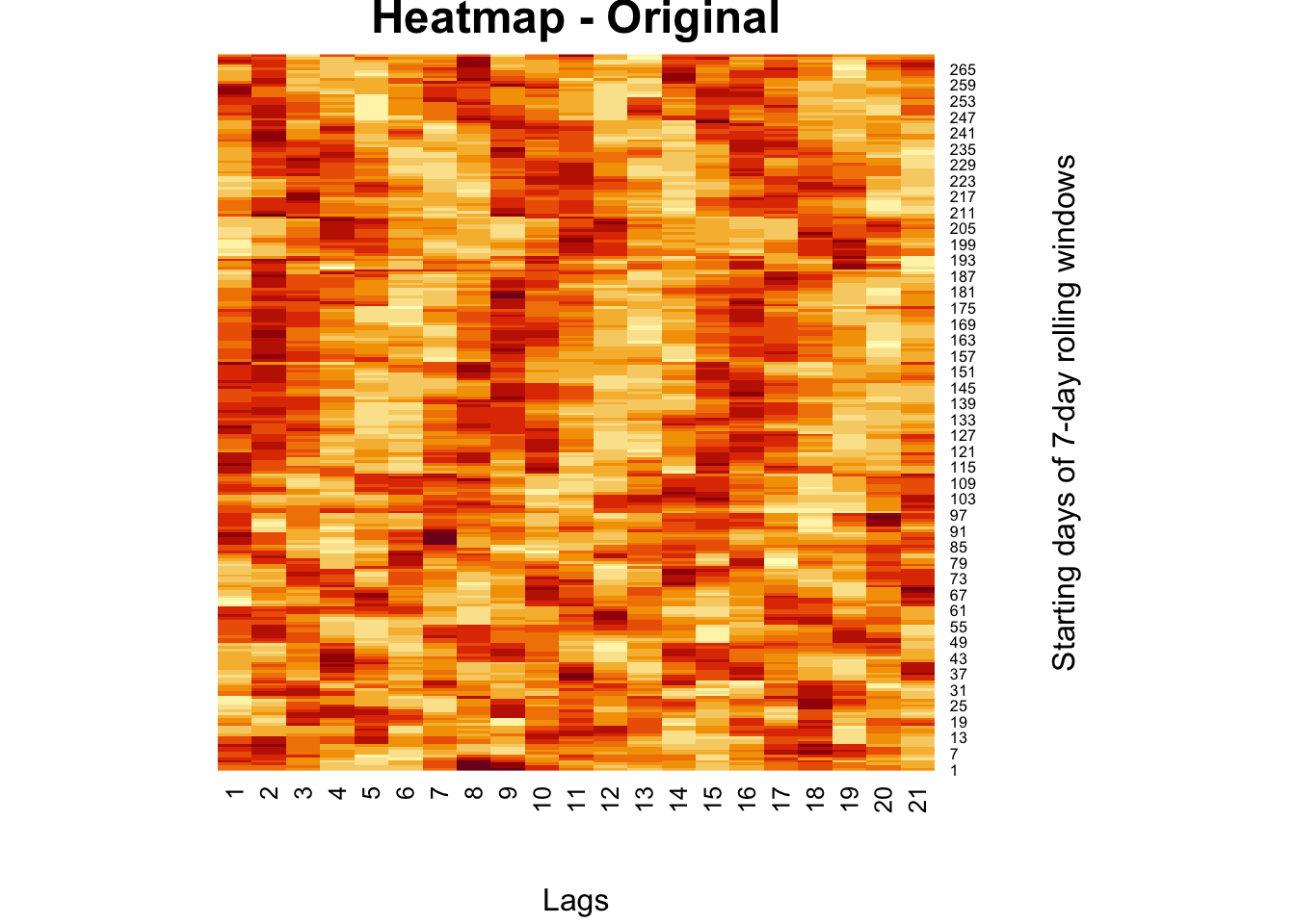
There are many examples on the Internet for real image compression, but we apply rank approximation to a heatmap from our own work. The heatmap shows moving-window partial correlations between daily positivity rates (Covid-19) and mobility restrictions for different time delays (days, “lags”)

comt <- readRDS("comt.rds")

heatmap(
  comt,
  Colv = NA,
  Rowv = NA,
  main = "Heatmap - Original",
  xlab = "Lags",
  ylab = "Starting days of 7-day rolling windows"
)

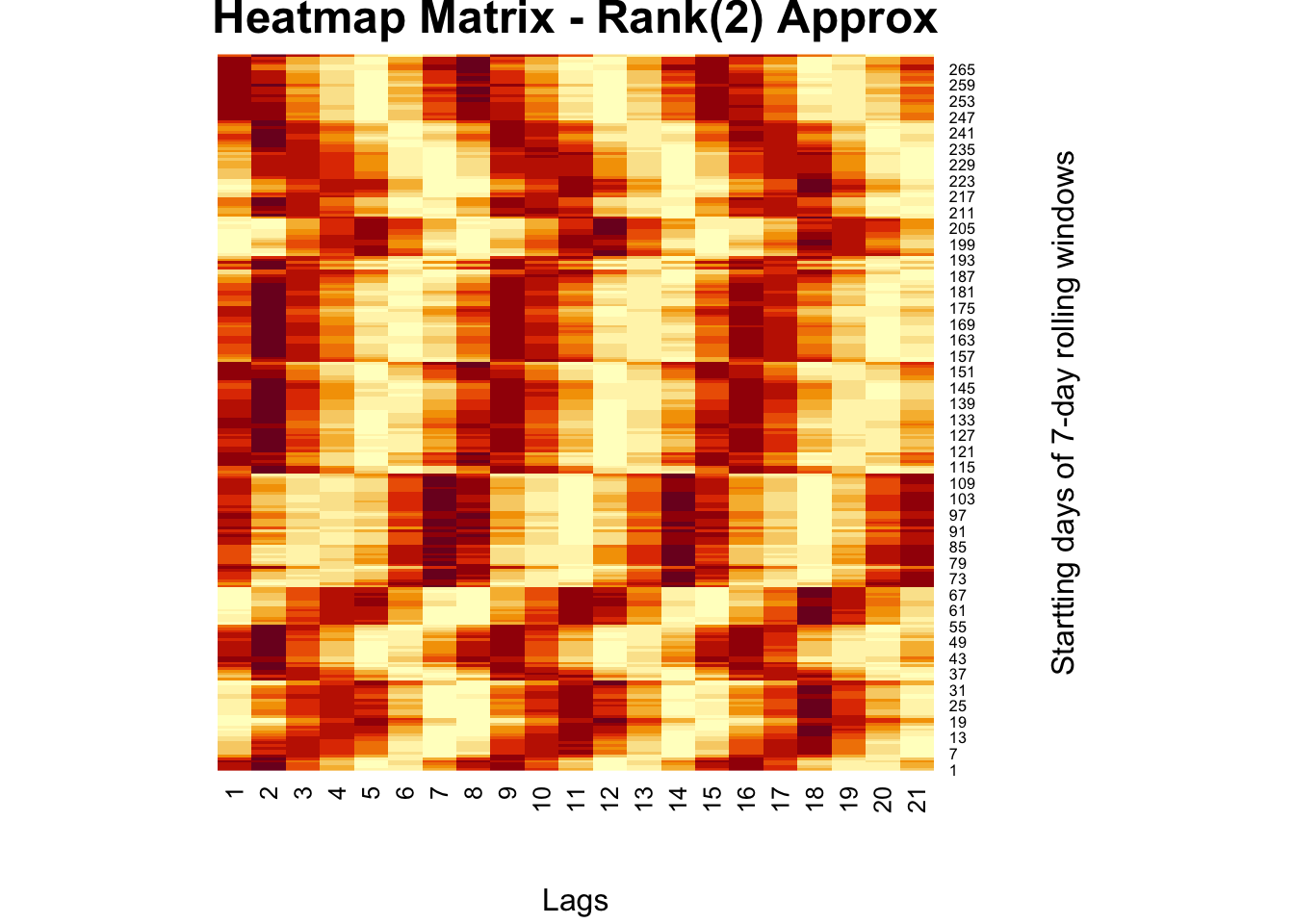
# Rank(2) with SVD
fck <- svd(comt)
r = 2
comt.re <-
  as.matrix(fck$u[, 1:r]) %*% diag(fck$d)[1:r, 1:r] %*% t(fck$v[, 1:r])

heatmap(
  comt.re,
  Colv = NA,
  Rowv = NA,
  main = "Heatmap Matrix - Rank(2) Approx",
  xlab = "Lags",
  ylab = "Startting days of 7-day rolling windows"
)

This Rank(2) approximation reduces the noise in the moving-window partial correlations so that we can see the clear trend about the delay in the effect of mobility restrictions on the spread.

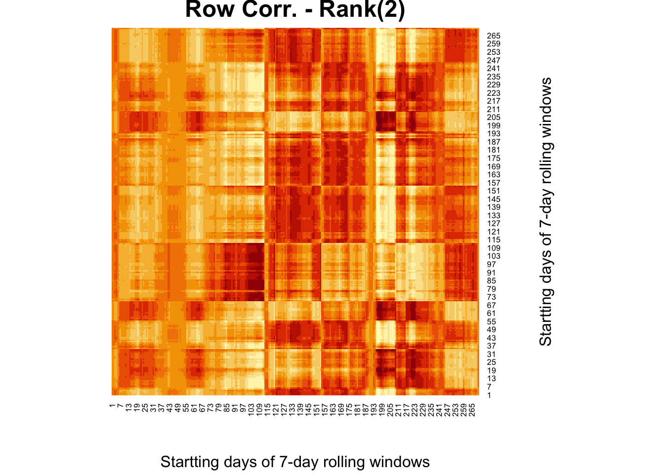
We change the order of correlations in the original heatmap, and make it row-wise correlations:

#XX' and X'X SVD
wtf <- comt %*% t(comt)
fck <- svd(wtf)
r = 2
comt.re2 <-
  as.matrix(fck$u[, 1:r]) %*% diag(fck$d)[1:r, 1:r] %*% t(fck$v[, 1:r])

heatmap(
  comt.re2,
  Colv = NA,
  Rowv = NA,
  main = "Row Corr. - Rank(2)",
  xlab = "Startting days of 7-day rolling windows",
  ylab = "Startting days of 7-day rolling windows"
)

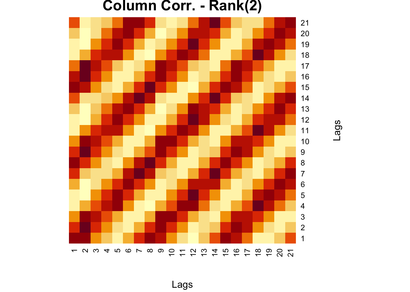
This is now worse than the original heatmap we had ealier. When we apply a Rank(2) approximation, however, we have a very clear picture:

wtf <- t(comt) %*% comt
fck <- svd(wtf)
r = 2
comt.re3 <-
  as.matrix(fck$u[, 1:r]) %*% diag(fck$d)[1:r, 1:r] %*% t(fck$v[, 1:r])

heatmap(
  comt.re3,
  Colv = NA,
  Rowv = NA,
  main = "Column Corr. - Rank(2)",
  xlab = "Lags",
  ylab = "Lags"
)

There is a series of great lectures on SVD and other matrix approximations by Steve Brunton at YouTube https://www.youtube.com/watch?v=nbBvuuNVfco.