Chapter 22 Grid search for ARIMA

Before we apply a cross validation approach to choose the model that has the minimum test error (out-sample), we would like to do a grid search for a seasonal ARIMA with \(d=1\), \(D=1\), and \(S=7\). We will report two outcomes: AICc and RMSE (root mean squared error).

#In-sample grid-search
p <- 0:3
q <- 0:3
P <- 0:3
Q <- 0:2

comb <- as.matrix(expand.grid(p, q, P, Q))

# We remove the unstable grids
comb <- as.data.frame(comb[-1,])
ind <- which(comb$Var1 == 0 & comb$Var2 == 0, arr.ind = TRUE)
comb <- comb[-ind,]
row.names(comb) <- NULL
colnames(comb) <- c("p", "q", "P", "Q")

aicc <- c()
RMSE <- c()

for (k in 1:nrow(comb)) {
  tryCatch({
    fit <- toronto %>%
      model(ARIMA(boxcases ~ 0 + pdq(comb[k, 1], 1, comb[k, 2])
                  + PDQ(comb[k, 3], 1, comb[k, 4])))
    wtf <- fit %>% glance
    res <- fit %>% residuals()
    aicc[k] <- wtf$AICc
    RMSE[k] <- sqrt(mean((res$.resid) ^ 2))
  }, error = function(e) {
  })
}

cbind(comb[which.min(aicc), ], "AICc" = min(aicc, na.rm = TRUE))

##    p q P Q     AICc
## 75 3 3 0 1 558.7747

cbind(comb[which.min(RMSE), ], "RMSE" = min(RMSE, na.rm = TRUE))

##     p q P Q      RMSE
## 165 3 3 2 2 0.6482865

Although we set the ARIMA without a constant, we could extend the grid with a constant. We can also add a line (ljung_box) that extracts and reports the Ljung-Box test for each model. We can then select the one that has a minimum AICc and passes the test.

We may not need this grid search as the Hyndman-Khandakar algorithm for automatic ARIMA modelling is able to do it for us very effectively (except for the Ljung-Box test for each model). We should note that the Hyndman-Khandakar algorithm selects the best ARIMA model for forecasting with the minimum AICc. In practice, we can apply a similar grid search with cross validation for selecting the best model that has the minimum out-of-sample prediction error without checking if it passes the Ljung-Box test or not. Here is a simple example:

#In-sample grid-search
p <- 0:3
q <- 0:3
P <- 0:3
Q <- 0:2

comb <- as.matrix(expand.grid(p, q, P, Q))

# We remove the unstable grids
comb <- as.data.frame(comb[-1,])
ind <- which(comb$Var1 == 0 & comb$Var2 == 0, arr.ind = TRUE)
comb <- comb[-ind, ]
row.names(comb) <- NULL
colnames(comb) <- c("p", "q", "P", "Q")

train <- toronto %>%
  filter_index( ~ "2020-11-14")

RMSE <- c()

for (k in 1:nrow(comb)) {
  tryCatch({
    amk <- train %>%
      model(ARIMA(boxcases ~ 0 + pdq(comb[k, 1], 1, comb[k, 2])
                  + PDQ(comb[k, 3], 1, comb[k, 4]))) %>%
      forecast(h = 7) %>%
      accuracy(toronto)
    RMSE[k] <- amk$RMSE
  }, error = function(e) {
  })
}

cbind(comb[which.min(RMSE), ], "RMSE" = min(RMSE, na.rm = TRUE))

##    p q P Q      RMSE
## 12 0 3 0 0 0.7937723

g <- which.min(RMSE)
toronto %>%
  model(ARIMA(boxcases ~ 0 + pdq(comb[g, 1], 1, comb[g, 2])
              + PDQ(comb[g, 3], 1, comb[g, 4]))) %>%
  forecast(h = 7) %>%
  autoplot(toronto, level = NULL)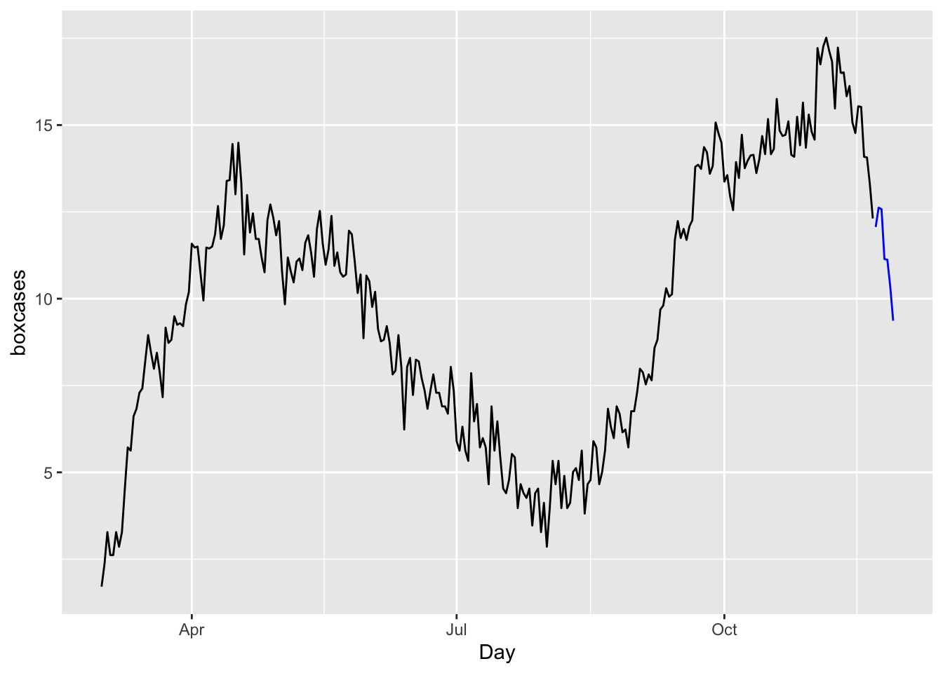

We will not apply h-step-ahead rolling-window cross-validations for ARIMA, which can be found in the post, Time series cross-validation using fable, by Hyndman (2021). However, when we have multiple competing models, we may not want to compare their predictive accuracy by looking at their error rates using only few out-of-sample observations. If we use rolling windows or continuously expanding windows, we can effectively create a large number of days tested within the data.