Chapter 18 Lasso
The penalty in ridge regression, \(\lambda \sum_{j} \beta_{j}^{2}\), will shrink all of the coefficients towards zero, but it will not set any of them exactly to zero. This may present a problem in model interpretation when the number of variables is quite large. One of the key advantages of Lasso is that it can set the coefficients of some features to exactly zero, effectively eliminating those features from the model.
By eliminating unnecessary or redundant features from the model, Lasso can help to improve the interpretability and simplicity of the model. This can be particularly useful when you have a large number of features and you want to identify the most important ones for predicting the target variable.
The lasso, a relatively recent alternative to ridge regression, minimizes the following quantity:
\[\begin{equation} \sum_{i=1}^{n}\left(y_{i}-\beta_{0}-\sum_{j=1}^{p} \beta_{j} x_{i j}\right)^{2}+\lambda \sum_{j=1}^{p}\left|\beta_{j}\right|=\operatorname{RSS}+\lambda \sum_{j=1}^{p}\left|\beta_{j}\right| \tag{18.1} \end{equation}\]
The lasso also shrinks the coefficient estimates towards zero. However, the \(\ell_{1}\) penalty, the second term of equation 18.1, has the effect of forcing some of the coefficient estimates to be exactly equal to zero when the tuning parameter \(\lambda\) is sufficiently large. Hence, the lasso performs variable selection. As a result, models generated from the lasso are generally much easier to interpret than those produced by ridge regression.
In general, one might expect lasso to perform better in a setting where a relatively small number of predictors have substantial coefficients and the remaining predictors have no significant effect on the outcome. This property is known as “sparsity”, because it results in a model with a relatively small number of non-zero coefficients. In some cases, Lasso can find a true sparsity pattern in the data by identifying a small subset of the most important features that are sufficient to accurately predict the target variable.
Now, we apply lasso to the same data, Hitters. Again, we will follow a similar way to compare ridge and lasso as in Introduction to Statistical Learning ((James et al. 2013)).
library(glmnet)
library(ISLR)
remove(list = ls())

data(Hitters)
df <- Hitters[complete.cases(Hitters$Salary), ]
X  <- model.matrix(Salary ~ ., df)[,-1]
y <- df$Salary

# Without a specific grid on lambda
set.seed(1)
train <- sample(1:nrow(X), nrow(X) * 0.5)
test <- c(-train)
ytest <- y[test]

# Ridge
set.seed(1)
ridge.out <- cv.glmnet(X[train,], y[train], alpha = 0)
yhatR <- predict(ridge.out, s = "lambda.min", newx = X[test,])
mse_r <- mean((yhatR - ytest)^2)

# Lasso
set.seed(1)
lasso.out <- cv.glmnet(X[train,], y[train], alpha = 1)
yhatL <- predict(lasso.out, s = "lambda.min", newx = X[test,])
mse_l <- mean((yhatL - ytest) ^ 2)

mse_r
## [1] 139863.2mse_l## [1] 143668.8Now, we will define our own grid search:
# With a specific grid on lambda + lm()
grid = 10 ^ seq(10, -2, length = 100)

set.seed(1)
train <- sample(1:nrow(X), nrow(X)*0.5)
test <- c(-train)
ytest <- y[test]

#Ridge
ridge.mod <- glmnet(X[train,], y[train], alpha = 0,
                    lambda = grid, thresh = 1e-12)
set.seed(1)
cv.outR <- cv.glmnet(X[train,], y[train], alpha = 0)
bestlamR <- cv.outR$lambda.min
yhatR <- predict(ridge.mod, s = bestlamR, newx = X[test,])
mse_R <- mean((yhatR - ytest) ^ 2)

# Lasso
lasso.mod <- glmnet(X[train,], y[train], alpha = 1,
                    lambda = grid, thresh = 1e-12)
set.seed(1)
cv.outL <- cv.glmnet(X[train,], y[train], alpha = 1)
bestlamL <- cv.outL$lambda.min
yhatL <- predict(lasso.mod, s = bestlamL, newx = X[test,])
mse_L <- mean((yhatL - ytest) ^ 2)

mse_R
## [1] 139856.6mse_L## [1] 143572.1Now, we apply our own algorithm:
grid = 10 ^ seq(10, -2, length = 100)
MSPE <- c()
MMSPE <- c()

for(i in 1:length(grid)){
  for(j in 1:100){
    set.seed(j)
    ind <- unique(sample(nrow(df), nrow(df), replace = TRUE))

    train <- df[ind, ]
    xtrain <- model.matrix(Salary ~ ., train)[,-1]
    ytrain <- df[ind, 19]

    test <- df[-ind, ]
    xtest <- model.matrix(Salary~., test)[,-1]
    ytest <- df[-ind, 19]

    model <- glmnet(xtrain, ytrain, alpha = 1,
                    lambda = grid[i], thresh = 1e-12)
    yhat <- predict(model, s = grid[i], newx = xtest)
    MSPE[j] <- mean((yhat - ytest) ^ 2)
    }
  MMSPE[i] <- mean(MSPE)
}

min(MMSPE)
## [1] 119855.1grid[which.min(MMSPE)]## [1] 2.656088plot(log(grid), MMSPE, type="o", col = "red", lwd = 3)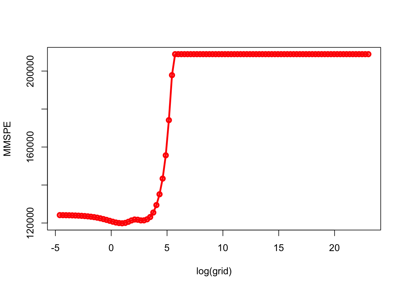
What are the coefficients?
coef_lasso <- coef(model, s=grid[which.min(MMSPE)], nonzero = T)
coef_lasso
## NULLWe can also try a classification problem with LPM or Logistic regression when the response is categorical. If there are two possible outcomes, we use the binomial distribution, else we use the multinomial.