Chapter 26 Rank(r) Approximations
SVD can also be used for rank approximations a.k.a. matrix approximations. Since \(\mathbf{A=U \Sigma V^{\top}}\) can be written as
\[ =\sigma_{1} u_{1} v_{1}^{\top}+\sigma_{2} u_{2} v_{2}^{\top}+\ldots+\sigma_{n} u_{n} v_{n}^{\top}+ 0 \] Each term in this equation is a Rank 1 matrix: \(u_1\) is \(n \times 1\) column vector and \(v_1\) is \(1 \times n\) row vector. Hence these are the only orthogonal entries in the resulting matrix, hence Rank1. Therefore, the first term with \(\sigma_1\) is a Rank 1 \(n \times n\) matrix. All other terms have the same dimension. Since \(\sigma\)s are ordered, the first term is the carries the most information. So Rank 1 approximation is taking only the first term and ignoring the others. Here is a simple example:
#rank-one approximation
#http://cs.brown.edu/courses/cs053/current/slides/12-01-2017.pdf
#https://cran.r-project.org/web/packages/matlib/vignettes/eigen-ex1.html

A <- matrix(c(1,5,4,2), 2 ,2)
A
## [,1] [,2]
## [1,] 1 4
## [2,] 5 2v1 <- matrix(eigen(t(A)%*%(A))$vector[,1], 1, 2)
sigma <- sqrt(eigen(t(A)%*%(A))$values[1])
u1 <- matrix(eigen(A%*%t(A))$vector[,1], 2, 1)
Atilde <- sigma*u1%*%v1
Atilde## [,1] [,2]
## [1,] -2.560369 -2.069843
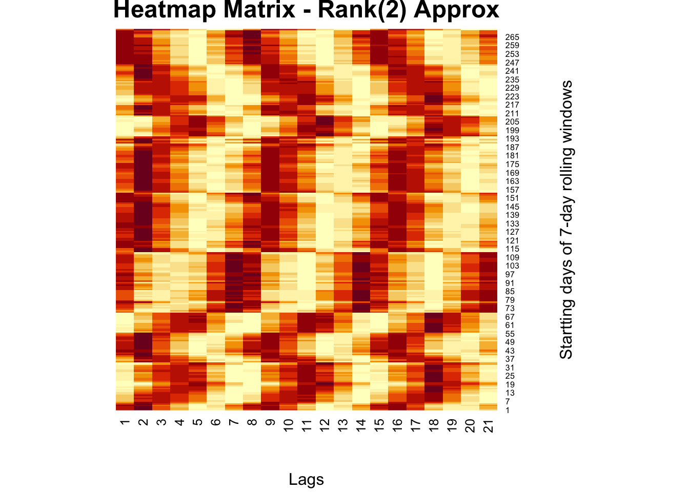
## [2,] -4.001625 -3.234977And, Rank 2 approximation can be obtained by adding the first 2 terms and so on. As we add more terms we can get the full information in the data. But often times, we truncate the ranks at \(r\) by removing the terms with small \(sigma\). This is also called noise reduction.
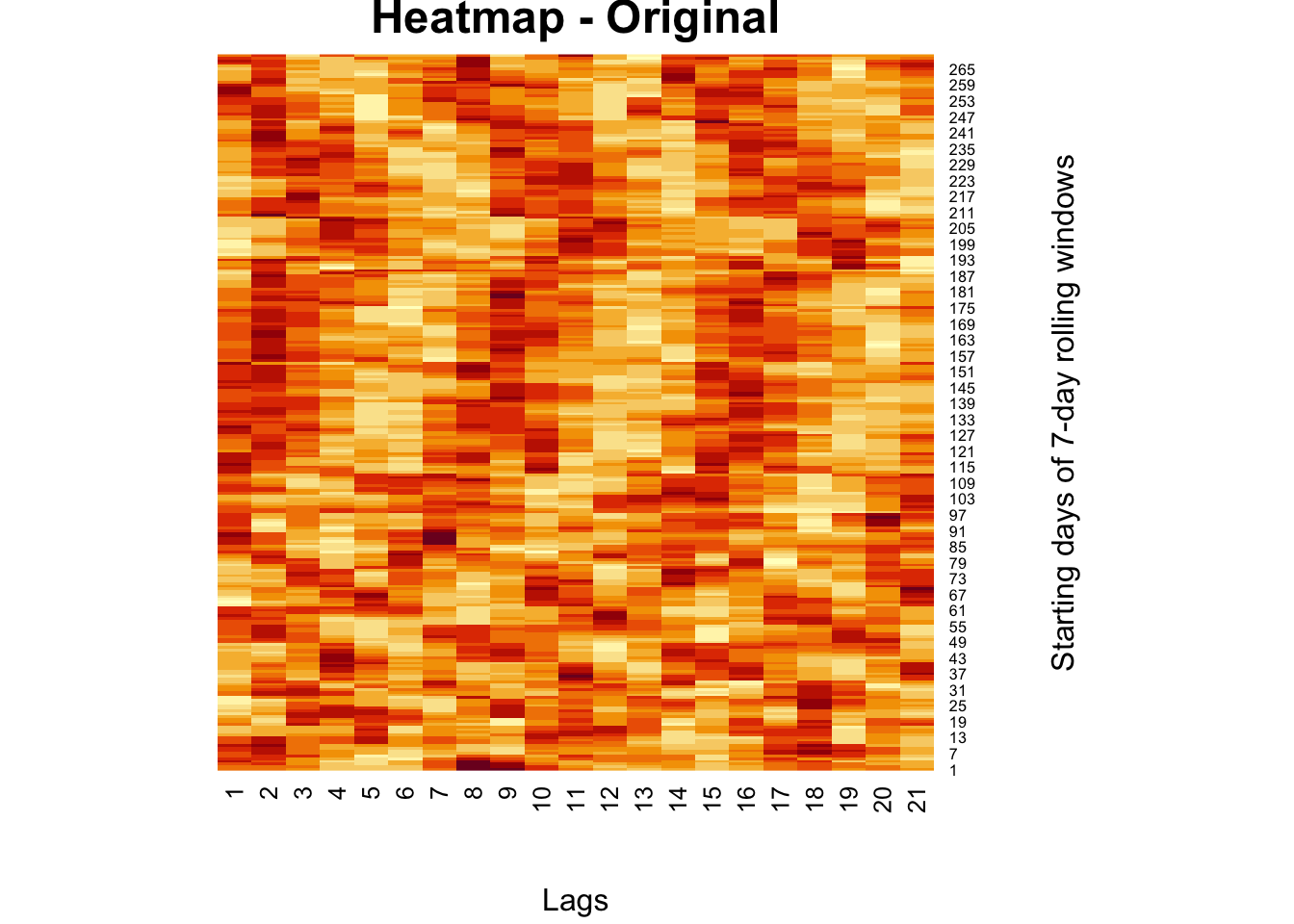
Here is an example for an image compression for a matrix from our own work (Graphical Network Analysis of COVID-19 Spread). A better example for an image can be found in the Github repo of package rsvd Tiger (Erichson et al. 2019):
comt <- readRDS("comt.rds")

heatmap(comt, Colv = NA, Rowv = NA,
        main = "Heatmap - Original",
        xlab = "Lags", ylab = "Starting days of 7-day rolling windows")
# Regular SVD
fck <-svd(comt)
r = 2
comt.re <- as.matrix(fck$u[,1:r])%*%diag(fck$d)[1:r,1:r]%*%t(fck$v[,1:r])

heatmap(comt.re, Colv = NA, Rowv = NA,
        main = "Heatmap Matrix - Rank(2) Approx",
        xlab = "Lags", ylab = "Startting days of 7-day rolling windows")
#XX' and X'X SVD
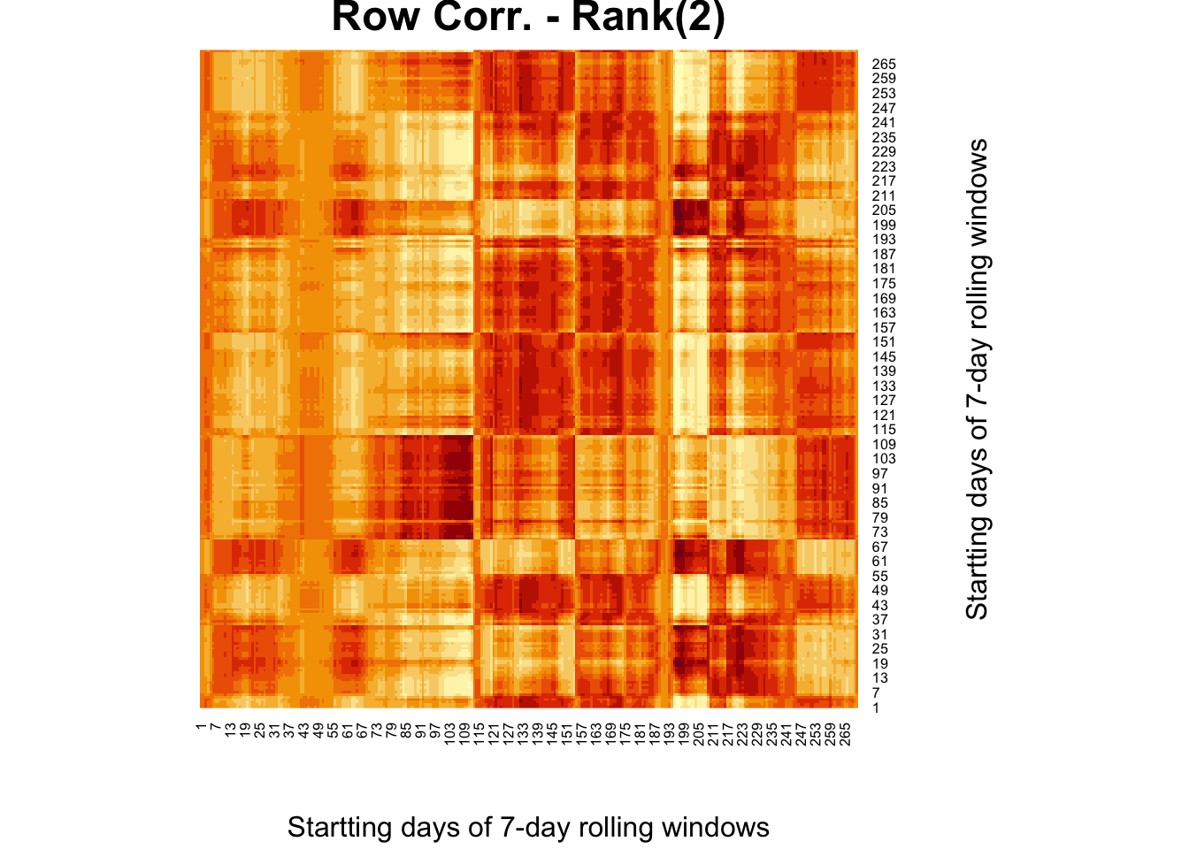
wtf <- comt%*%t(comt)
fck <-svd(wtf)
r = 2
comt.re2 <- as.matrix(fck$u[,1:r])%*%diag(fck$d)[1:r,1:r]%*%t(fck$v[,1:r])

heatmap(comt.re2, Colv = NA, Rowv = NA,
        main = "Row Corr. - Rank(2)",
        xlab = "Startting days of 7-day rolling windows",
        ylab = "Startting days of 7-day rolling windows")
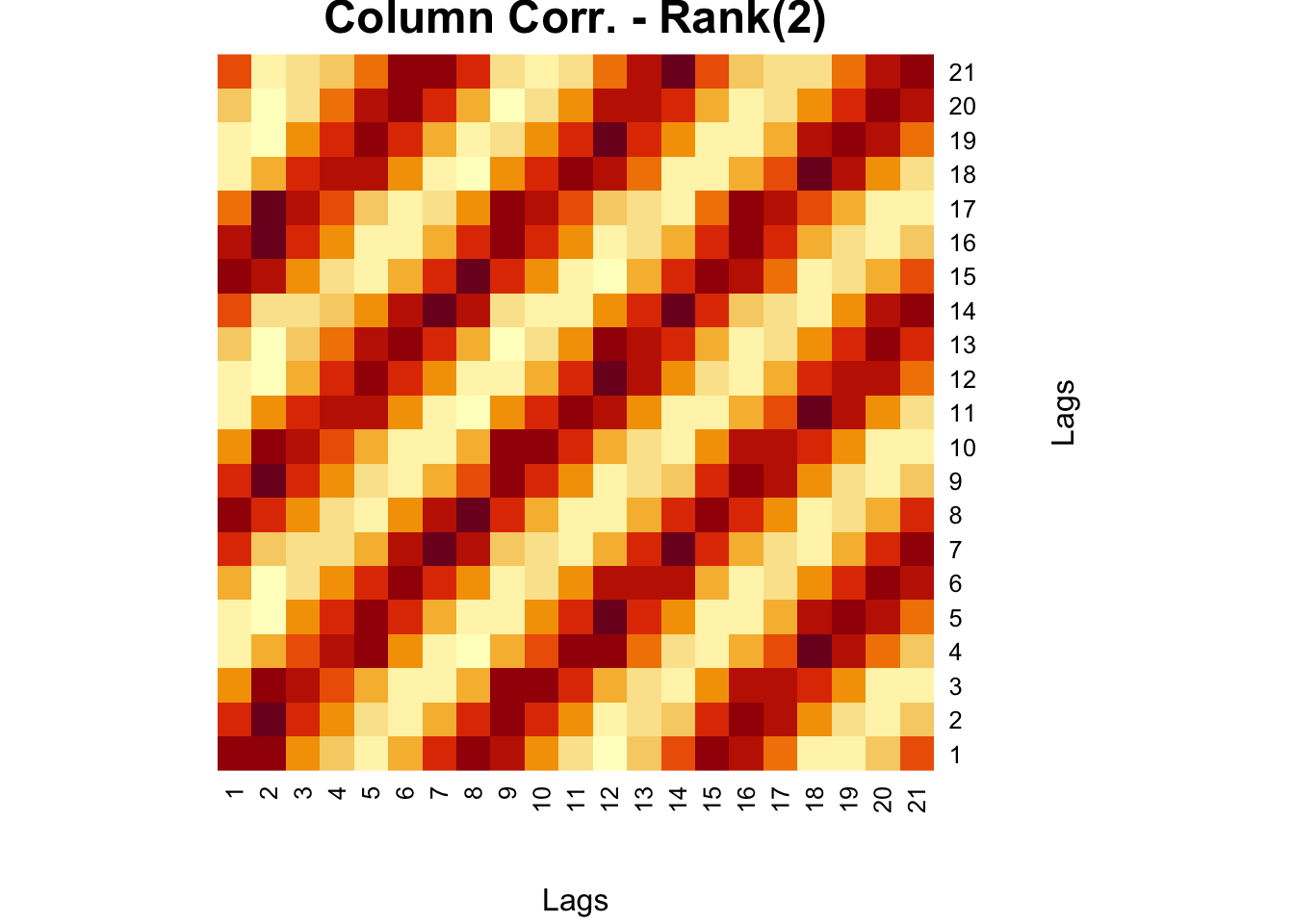
wtf <- t(comt)%*%comt
fck <-svd(wtf)
r = 2
comt.re3 <- as.matrix(fck$u[,1:r])%*%diag(fck$d)[1:r,1:r]%*%t(fck$v[,1:r])

heatmap(comt.re3, Colv = NA, Rowv = NA,
        main = "Column Corr. - Rank(2)",
        xlab = "Lags", ylab = "Lags")
There is a series of lectures on SVD by Steve Brunton at YouTube (Brunton 2020b) that you can benefit from greatly!