Chapter 7 Smoothing
We can define \(Y_i\) with a following model:
\[ Y_{i}=f\left(x_{i}\right)+\varepsilon_{i} \]
We do not want to (and cannot) predict \(Y_i\) as we don’t know the random part, the “noise” \(\epsilon_i\). If we predict \(f(x)\) well, it would give us a good approximation about \(Y_i\). Hence we need to know the best \(f(x)\). Nonparametric estimations can also be used for recovering \(f(x)\), which is called “smoothing” when the outcome variable is quantitative. In general, the purposes of smoothing is two-fold: building a forecasting model by smoothing and learning the shape of the trend embedded in the data (\(Y\)). You can think of smoothing as process that reduces the effect of noise in the data.
We will use several datasets from MASS. The mcycle dataset (from the MASS package) contains \(n=133\) pairs of time points (in ms) and observed head accelerations (in g) that were recorded in a simulated motorcycle accident. We will several smoothing methods to explore the relationship between time and acceleration. Fist, let’s visualize the relationship between time \((X)\) and acceleration \((Y)\) and see if we can assume that \(f(x_i)\) is a linear function of time:
library(tidyverse)
library(MASS)
data(mcycle)
head(mcycle)
## times accel
## 1 2.4 0.0
## 2 2.6 -1.3
## 3 3.2 -2.7
## 4 3.6 0.0
## 5 4.0 -2.7
## 6 6.2 -2.7plot(mcycle$times, mcycle$accel,
cex.axis = 0.75, cex.main = 0.8)
#Let’s use linear regression
lines(mcycle$times, predict(lm(accel ~ times, mcycle)), lwd = 2, col = "red")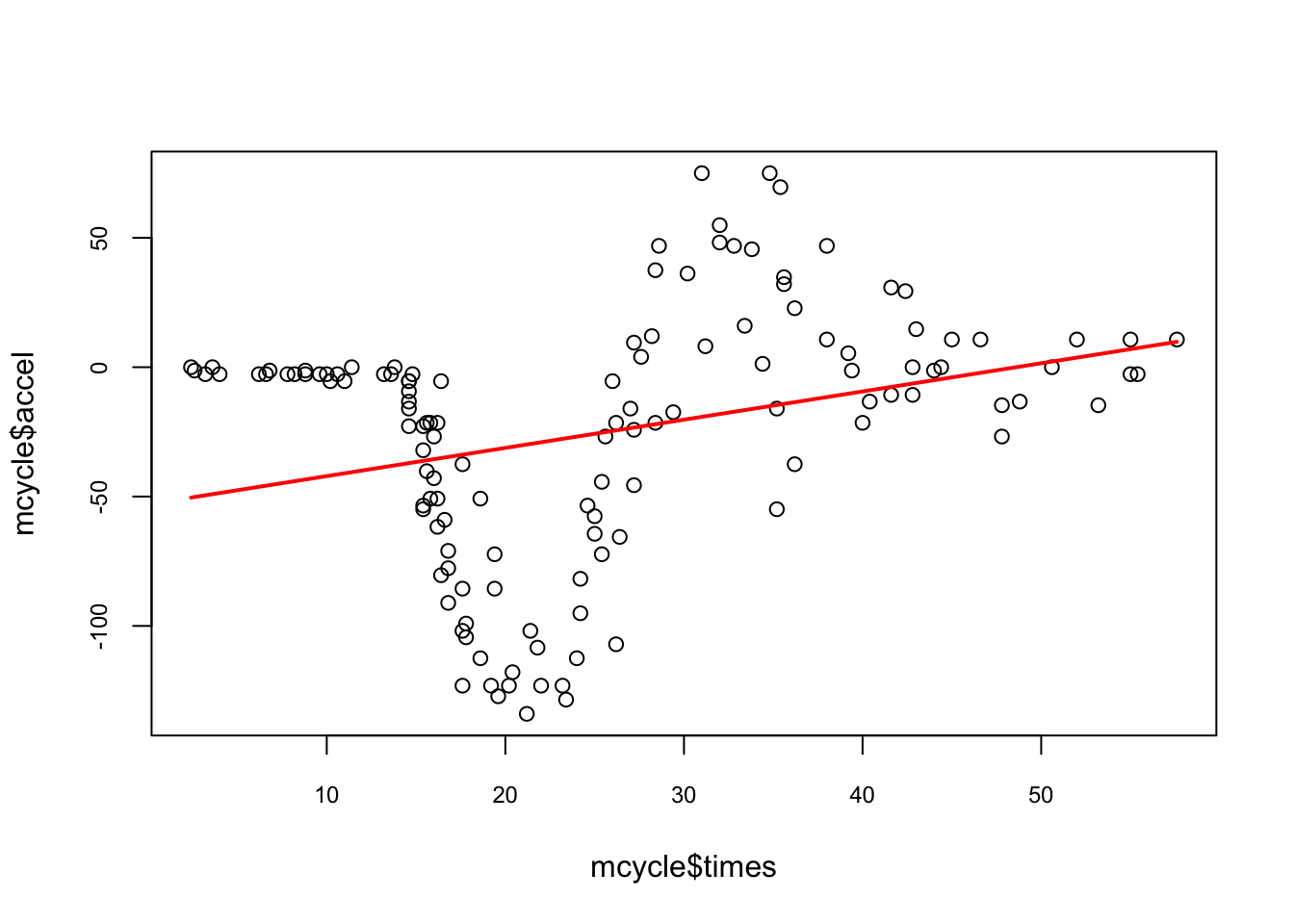
The line does not appear to describe the trend very well. Let’s try an alternative model:
7.1 Using bins
As we have seen before, the main idea is to group data points into bins (equal size) in which the value of \(f(x)\) can be assumed to be constant. We can consider this assumption realistic because we consider \(f(x)\) is almost constant in small windows of time. After deciding the window size (say, 10ms), we find out how many observations (\(Y_i\)) we have in those 10-ms windows. We can calculate the number of observations in a 10-ms window centered around \(x_i\) satisfying the following condition:
\[ \left(x-\frac{10}{2}<x_{i}<x+\frac{10}{2}\right) \] When we apply condition such as this for each observation of \(x_i\), we create a moving 10-ms window. Note that the window is established by adding half of 10ms to \(x_i\) to get the forward half and subtracting it from \(x_i\) to get the backward half. When we identify all the observations in each window, we estimate \(f(x)\) as the average of the \(Y_i\) values in that window. If we define \(A_0\) as the set of indexes in each window and \(N_0\) as the number of observation in each window, with our data, computing \(f(x)\) can be expressed as,
\[\begin{equation} \hat{f}\left(x_{0}\right)=\frac{1}{N_{0}} \sum_{i \in A_{0}} Y_{i}, \tag{7.1} \end{equation}\]
We build an estimate of the underlying curve. Here is its application to our data:
#With ksmooth() Pay attention to "box"
fit1 <- with(mcycle, ksmooth(times, accel, kernel = "box", bandwidth = 7))
fit2 <- with(mcycle, ksmooth(times, accel, kernel = "box", bandwidth = 10))
fit3 <- with(mcycle, ksmooth(times, accel, kernel = "box", bandwidth = 21))


plot(mcycle$times, mcycle$accel,
     xlab = "Time (ms)", ylab = "Acceleration (g)")
lines(mcycle$times,  fit1$y, lwd = 2, col = "blue")
lines(mcycle$times,  fit2$y, lwd = 2, col = "red")
lines(mcycle$times,  fit3$y, lwd = 2, col = "green")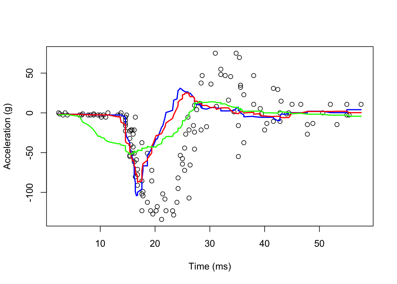
As you can see, even if we use a shorter bandwidth, the lines are quite wiggly.
7.2 Kernel smoothing
We can take care of this by taking weighted averages that give the center points more weight than far away points.
#With ksmooth() Pay attention to "box"
fit1 <- with(mcycle, ksmooth(times, accel, kernel = "normal", bandwidth = 7))
fit2 <- with(mcycle, ksmooth(times, accel, kernel = "normal", bandwidth = 10))
fit3 <- with(mcycle, ksmooth(times, accel, kernel = "normal", bandwidth = 21))


plot(mcycle$times, mcycle$accel,
     xlab = "Time (ms)", ylab = "Acceleration (g)")
lines(mcycle$times,  fit1$y, lwd = 2, col = "blue")
lines(mcycle$times,  fit2$y, lwd = 2, col = "red")
lines(mcycle$times,  fit3$y, lwd = 2, col = "green")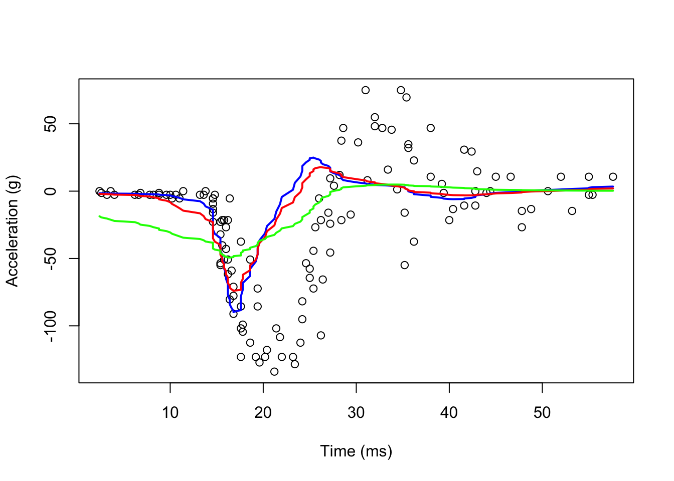
Now they look smoother. There are several functions in R that implement bin smoothers. One example is ksmooth, shown above. In practice, however, we typically prefer methods that are slightly more complex than fitting a constant. Methods such as loess, which we explain next, improve on this.
7.3 Locally weighted regression loess()
A limitation of the bin smoother approach by ksmooth() is that we need small windows for the approximately constant assumptions to hold. Now loess() permits us to consider larger window sizes.
#With loess()
fit1 <- loess(accel ~ times, degree = 1, span = 0.1, mcycle)
fit2 <-loess(accel ~ times, degree = 1, span = 0.9, mcycle)

summary(fit1)
## Call:
## loess(formula = accel ~ times, data = mcycle, span = 0.1, degree = 1)
##
## Number of Observations: 133
## Equivalent Number of Parameters: 18.57
## Residual Standard Error: 22.93
## Trace of smoother matrix: 22.01 (exact)
##
## Control settings:
## span : 0.1
## degree : 1
## family : gaussian
## surface : interpolate cell = 0.2
## normalize: TRUE
## parametric: FALSE
## drop.square: FALSEplot(mcycle$times, mcycle$accel,
xlab = "Time (ms)", ylab = "Acceleration (g)")
lines(mcycle$times, fit1$fitted, lwd = 2, col = "blue")
lines(mcycle$times, fit2$fitted, lwd = 2, col = "red")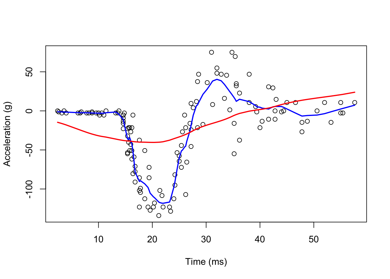
It seems the “blue” line is better than the “red” line. We can make our windows even larger by fitting parabolas instead of lines.
fit1 <- loess(accel ~ times, degree = 1, span = 0.1, data = mcycle)
fit2 <-loess(accel ~ times, degree = 2, span = 0.1, data = mcycle)

plot(mcycle$times, mcycle$accel,
     xlab = "Time (ms)", ylab = "Acceleration (g)")
lines(mcycle$times,  fit1$fitted, lwd = 2, col = "blue")
lines(mcycle$times,  fit2$fitted, lwd = 2, col = "green")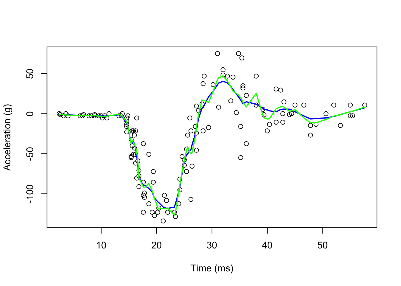
7.4 Smooth Spline Regression
We can also use npreg package with ss() function for automated smooth splines
library(npreg)

mod.ss <- with(mcycle, ss(times, accel))
mod.ss
##
## Call:
## ss(x = times, y = accel)
##
## Smoothing Parameter spar = 0.1585867 lambda = 8.337283e-07
## Equivalent Degrees of Freedom (Df) 12.20781
## Penalized Criterion (RSS) 62034.66
## Generalized Cross-Validation (GCV) 565.4684summary(mod.ss)##
## Call:
## ss(x = times, y = accel)
##
## Residuals:
## Min 1Q Median 3Q Max
## -76.7951 -12.5654 -0.8346 12.5823 50.5576
##
## Approx. Signif. of Parametric Effects:
## Estimate Std. Error t value Pr(>|t|)
## (Intercept) -14.234 2.313 -6.154 1.018e-08 ***
## x 9.549 21.603 0.442 6.593e-01
## ---
## Signif. codes: 0 '***' 0.001 '**' 0.01 '*' 0.05 '.' 0.1 ' ' 1
##
## Approx. Signif. of Nonparametric Effects:
## Df Sum Sq Mean Sq F value Pr(>F)
## s(x) 10.21 210130 20585.3 40.08 0 ***
## Residuals 120.79 62035 513.6
## ---
## Signif. codes: 0 '***' 0.001 '**' 0.01 '*' 0.05 '.' 0.1 ' ' 1
##
## Residual standard error: 22.66 on 120.8 degrees of freedom
## Multiple R-squared: 0.7999, Adjusted R-squared: 0.7801
## F-statistic: 41.21 on 11.21 and 120.8 DF, p-value: <2e-16plot(mod.ss, xlab = "Time (ms)", ylab = "Acceleration (g)", col = "orange")
rug(mcycle$times) # add rug to plot for the precise location of each point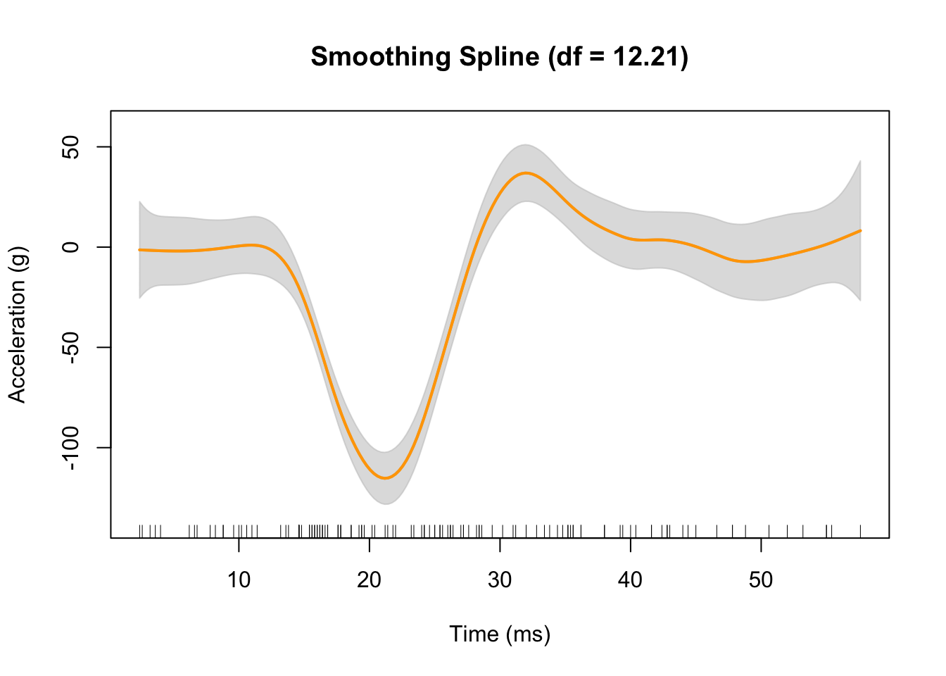
The gray shaded area denotes a 95% Bayesian “confidence interval” for the unknown function.
7.5 Multivariate Loess
Loess can handle up to 4 predictor variables. But when it’s more than two, it’s always advisable to use additive models either GAM or MARS. Let’s try loess() with 3 variables. This dataset was produced from US economic time series data available from St.Louis Federal Reserve. It’s a data frame with 478 rows and 6 variables: psavert, personal savings rate; pce, personal consumption expenditures, in billions of dollars; unemploy, number of unemployed in thousands, uempmed median duration of unemployment, in weeks; and pop total population, in thousands. Although we have a time variable, date, let’s create an index for time.
data(economics, package="ggplot2")
str(economics)
## spc_tbl_ [574 × 6] (S3: spec_tbl_df/tbl_df/tbl/data.frame)
## $ date : Date[1:574], format: "1967-07-01" "1967-08-01" ...
## $ pce : num [1:574] 507 510 516 512 517 ...
## $ pop : num [1:574] 198712 198911 199113 199311 199498 ...
## $ psavert : num [1:574] 12.6 12.6 11.9 12.9 12.8 11.8 11.7 12.3 11.7 12.3 ...
## $ uempmed : num [1:574] 4.5 4.7 4.6 4.9 4.7 4.8 5.1 4.5 4.1 4.6 ...
## $ unemploy: num [1:574] 2944 2945 2958 3143 3066 ...economics$index <- 1:nrow(economics)
fit1 <- loess(uempmed ~ index, data=economics, span=0.5) # 40% smoothing span
plot(economics$index, economics$uempmed,
cex.axis = 0.75, cex.main = 0.8)
lines(economics$index, fit1$fitted, lwd = 2, col = "red")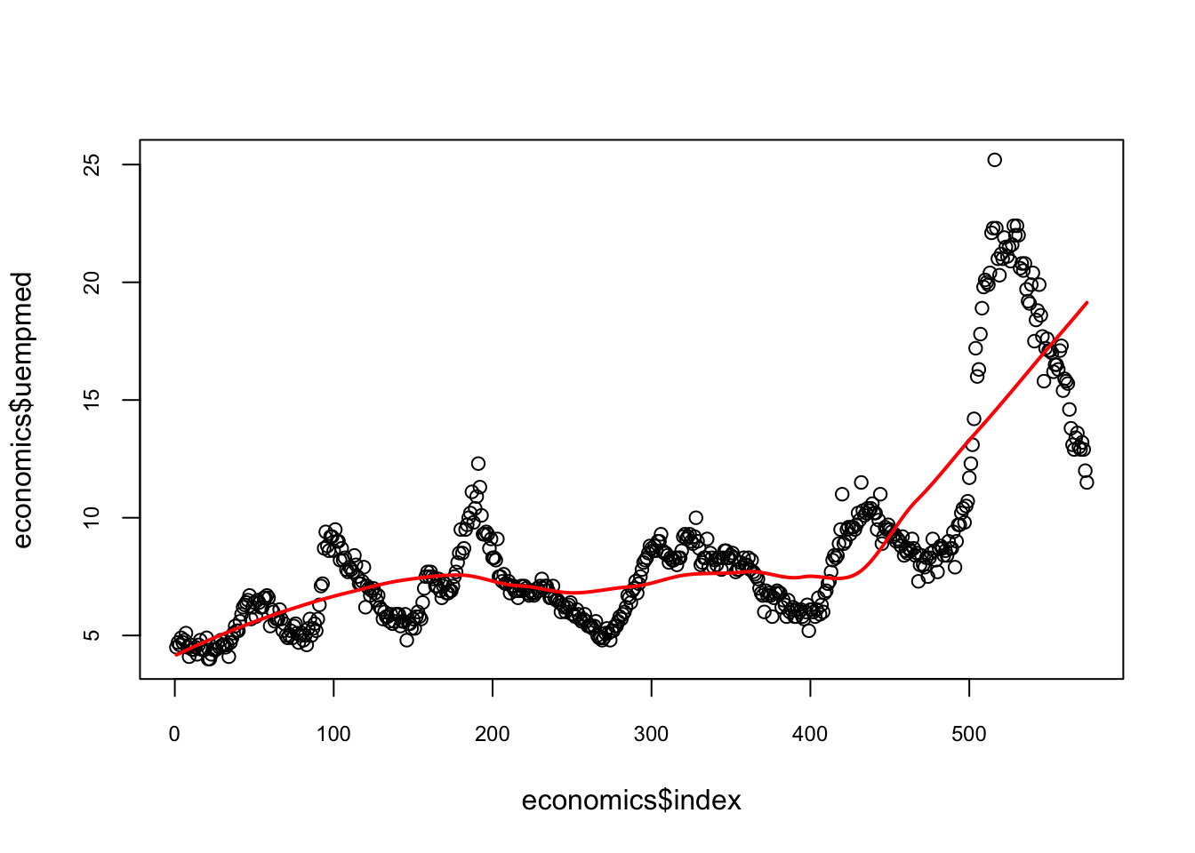
#Now more predictors
fit2 <- loess(uempmed ~ pce + psavert +pop,
              data=economics, span=1)

RRSS_2 <- sqrt(sum((fit2$residuals)^2))
RRSS_2
## [1] 121.3815